ZeRO to Hero: Adaptive Optimizers From Scratch

In the last blog we developed our intuition for optimization, developed a few momentum-based optimizers, and evaluated their performance on optimizing a single function. In this installation, we will continue showcasing how to build these optimizers from scratch.

However; rather than focusing on toy examples, we will directly be jumping into neural networks — specifically we will be building on top of the Makemore code that was developed in Andrej Karpathy’s Neural Networks: Zero to Hero series. If you haven’t seen it yet, it’s highly recommended to start with that first. Thankfully the Makemore code will serve as a proper basis for us, so I’ve created a fork that we can use to store everything we’ve discussed in here: osilkin98/makemore.

In this blog, we will develop our own adaptive learning rate optimzers such as Adagrad, RMSProp, Adam, and AdamW which we will use to train a name-generating Transformer model.

Setting up the repo

We will train Andrej Karpathy’s GPT-2 implementation on the names.txt dataset and compare how it performs against the optimizers we have built thus far.

To setup this example, you can clone the osilkin98/makemore GitHub repo and install it within a Python virtual environment:

# clone the repo
git clone https://github.com/osilkin98/makemore
cd makemore

# create a new virtual environment and install the necessary dependencies
python -m venv venv
source venv/bin/activate
pip install torch

Objective: Our objective with this repo will be to train the model until we begin over-fitting or we reach 100,000 steps.

Recap of previous work

Let’s quickly cover the optimizers from the previous blog and refine our work.

We will create a base Optimizer class for all of these optimizers to inherit for simplicity of our code:

class Optimizer:
  def __init__(self):
    self.params = []

  def zero_grad(self, set_to_none=True):
    # we respect `set_to_none` for pytorch compatibility
    for p in self.params:
      if set_to_none:
        p.grad = None
      else:
        p.grad.data = torch.zeros_like(p.data)

  def step(self):
    raise NotImplementedError()

Recall that in our previous blog we implemented few optimizers: SGD, SGD + Momentum, and Nesterov’s Accelerated Gradient. It turns out that we can actually combine the implementations a bit. Recall that basic SGD resembled the following:

class SGD(Optimizer):
  def __init__(self, params: List[Parameter], lr=1e-1):
    super().__init__()
    self.params = [p for p in params]
    self.lr = lr

  @torch.no_grad()
  def step(self):
    # very simple optimization step
    for p in self.params:
      p.data = p.data - self.lr * p.grad.data

We can combine this with momentum by adding a momentum argument to the __init__ method and making the necessary calculations & memory usage only be activated once a non-zero momentum is passed:

# now this can handle both naive SGD and momentum-based
class SGD(Optimizer):
  def __init__(self, params: List[Parameter], lr=1e-1, momentum: float = 0.0):
    super().__init__()
    self.params = [p for p in params]
    self.velocity = [None for _ in self.params] 
    self.lr = lr
    self.momentum = momentum

  @torch.no_grad()
  def step(self):
    # very simple optimization step
    for i, p in enumerate(self.params):
      grad = p.grad.data 
      if self.momentum > 0:
        # will only activate when non-zero momentum was provided
        if self.velocity[i] is None:
          self.velocity[i] = grad.clone().detach()
        else:
          self.velocity[i] = self.momentum * self.velocity[i] + grad
        grad = self.velocity[i]
      p.data = p.data - self.lr * grad

Now recall that in our NAG implementation, we simply had the parameter data update rule as:

p.data = p.data - self.lr * (p.grad.data + self.velocity[i] * self.momentum)

Where at this point self.velocity[i] already contained the following data:

self.velocity[i] = self.velocity[i] * self.momentum + p.grad.data

Therefore, we can simply add a nesterov flag to the class and use it to toggle what value grad stores when we perform the update rule:

 class SGD(Optimizer):
-  def __init__(self, params: List[Parameter], lr=1e-1, momentum: float = 0.0):
+  def __init__(self, params: List[Parameter], lr=1e-1, momentum: float = 0.0, nesterov = False):
     self.params = [p for p in params]
     self.velocity = [None for _ in self.params] 
     self.lr = lr
     self.momentum = momentum
+    self.nesterov = nesterov
 
   @torch.no_grad()
   def step(self):
     # very simple optimization step
     for i, p in enumerate(self.params):
       grad = p.grad.data 
       if self.momentum > 0:
         # will only activate when non-zero momentum was provided
         if self.velocity[i] is None:
           self.velocity[i] = grad.clone().detach()
         else:
           self.velocity[i] = self.momentum * self.velocity[i] + grad
         grad = self.velocity[i]
+        if self.nesterov:
+          grad = grad + self.velocity[i] * self.momentum
+        else:
+          grad = self.velocity[i]
       p.data = p.data - self.lr * grad

And just like that, we have effectively recreated what exists today in PyTorch for the SGD optimizer. The only thing we’re currently missing is the weight decay. But we will add that later 😉.

For now, we consider the following implementation of SGD to be the final one which we will use for this blog:

class SGD(Optimizer):
    def __init__(self, params: List[Parameter], lr=1e-1, momentum: float = 0.0, nesterov = False):
        self.params = [p for p in params]
        self.velocity = [None for _ in self.params] 
        self.lr = lr
        self.momentum = momentum
        self.nesterov = nesterov

    @torch.no_grad()
    def step(self):
        # very simple optimization step
        for i, p in enumerate(self.params):
            grad = p.grad.data 
            if self.momentum > 0:
                # will only activate when non-zero momentum was provided
                if self.velocity[i] is None:
                    self.velocity[i] = grad.clone().detach()
                else:
                    self.velocity[i] = self.momentum * self.velocity[i] + grad
                grad = self.velocity[i]
                if self.nesterov:
                    grad = grad + self.velocity[i] * self.momentum
                else:
                    grad = self.velocity[i]
            p.data = p.data - self.lr * grad

Preparing the repo

In order for us to test the optimizers, we’ll need to update the Makemore repo to export some extra visualizations and also provide the ability for us to select our own optimizers.

Providing Optimizer Selection

In order for us to test various optimizers, we’ll need to modify the makemore.py file to contain a switch to select the optimizers we’ll implement. We will also need to update the argument parser to accept the parameters that we’ll be passing to control the optimizers.

To allow us to select the optimizers, we’ll need to add an --optimizer flag and then parse it inside of the training script:

# optimization
parser.add_argument('--optimizer', type=str)

To parse this flag, let’s replace the optimizer = AdamW(...) initialization with a switch statement to parse the necessary optimizers:

# replaces the prior `optimizer = AdamW(...)` line
match args.optimizer:
    case "sgd":
        optimizer = SGD(model.parameters(), lr=args.learning_rate, momentum=args.momentum, nesterov=args.nesterov)
    case "adagrad":
        optimizer = Adagrad(model.parameters(), lr=args.learning_rate)
    case "rmsprop":
        optimizer = RMSProp(model.parameters(), lr=args.learning_rate, alpha=args.alpha)
    case "adam":
        optimizer = Adam(model.parameters(), lr=args.learning_rate, betas=(args.beta1, args.beta2))
    case "adamw":
        optimizer = AdamW(model.parameters(), lr=args.learning_rate, betas=(args.beta1, args.beta2), weight_decay=args.weight_decay)
    case _:
        raise ValueError(f'invalid optimizer selected: {args.optimizer}')

You might notice that we don’t have a few of these actually defined yet, but this is fine since Python is interpreted and therefore won’t actually error out unless you try to select one of the other optimizers.

Preparing visualization data

The makemore script currently uses TensorBoard to visualize the progress of training. We’ll be using this through the VSCode extension.

The current script is configured to export the training loss & validation loss as scalar values represented by the Loss/test and Loss/train values:

# evaluate the model
if step > 0 and step % 500 == 0:
    train_loss = evaluate(model, train_dataset, batch_size=100, max_batches=10)
    test_loss  = evaluate(model, test_dataset,  batch_size=100, max_batches=10)
    writer.add_scalar("Loss/train", train_loss, step)
    writer.add_scalar("Loss/test", test_loss, step)

These values are good for understanding our overall position in the training process, since we know that once the validation loss inflects back upward then we are now overfitting on our training dataset.

However, we’ll want to add two more scalars that will help us understand the state of our training progress: the gradient norm, commonly referred to as the gradnorm, as well as the learning rate norm which will be specific to the adaptive optimizers.

The gradnorm is defined as the L2 norm of the gradients and is used to understand whether or not our model has converged yet. If our gradnorm is relatively high then this indicates our model has still yet to fully converge, whereas a low grandorm tells us that we are very close to the minima.

The gradnorm is defined as the following equation:

$$\text{gradnorm}=\sqrt{\sum _{i=1}^N{\frac{\partial L({\theta }_t)}{\partial {\theta }_{t,i}}}^2}$$

Where:

• $L({\theta }_t)$ is the model loss across all parameters at time $t$
• ${\theta }_{t,i}$ represents the $i^{th}$ parameter at time $t$
• $N$ is the total number of parameters in the model

We can get this data by adding the following code to makemore.py:

@torch.no_grad()
def gradnorm(model: nn.Module) -> float:
    """
    Given a PyTorch model, computes the average of the gradnorm across all parameters.
    """
    grad_norms = []
    for p in model.parameters():
      grad_norms.append(p.grad.norm())
    return grad_norms

Then, in our main training loop, we can export the following scalars for TensorBoard:

# calculate gradnorm statistics
avg_gradnorm = 0 if not gradnorms else sum(gradnorms) / len(gradnorms)
max_gradnorm = max(gradnorms)
min_gradnorm = min(gradnorms)
total_gradnorm = sum(gradnorms)

# output various grandnorm scalars
writer.add_scalar("Gradnorm/average", avg_gradnorm, step)
writer.add_scalar("Gradnorm/max", max_gradnorm, step)
writer.add_scalar("Gradnorm/min", min_gradnorm, step)
writer.add_scalar("Gradnorm/total", total_gradnorm, step)

What this will do is help us understand, for all of the parameters in our model:

• Average gradnorm: the overall gradient norm we’re seeing in training
• Max gradnorm: Of all of our parameters, what’s the highest gradnrom that we’re seeing?
• Min gradnorm: Of all of our parameters, what’s the highest gradnrom that we’re seeing?
• Total gradnorm: The summation of all gradnorms throughout the network.

We’ll add the learning rate norm later, as it’s not needed for the initial tests.

Training the transformer

The model we will be training is Andrej Karpathy’s implementation of GPT-2 using default settings, amounting to roughly a 204,544 parameter model. We’ll train with each optimizer for exactly 100,000 steps.

The specific dataset we’re training on is a list of 32,033 names. I argue that this is a fairly easy dataset for a transformer to overfit on, while still having a sparse set of features perfect for a deep neural network to train on.

Stochastic Gradient Descent

Before we implement the other optimizers, let’s just grab a baseline of what our experience is training the transformer with SGD:

python3.11 makemore.py \
  --type='transformer' \
  --learning-rate=1e-3 \
  --optimizer='sgd' \
  --work-dir='out/transformer-sgd'

Using our new TensorBoard visualizations, we can view the training loss for Stochastic Gradient Descent under the default settings:

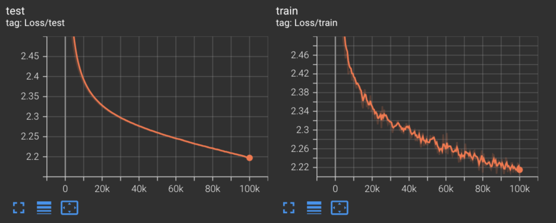
By viewing these graphs, we can see that after just 100,000 steps we’ve hit a training and test loss of 2.22 and 2.2 respectively.

Clearly we have more training that can be done under SGD, and the gradnorm charts tell a similar story:

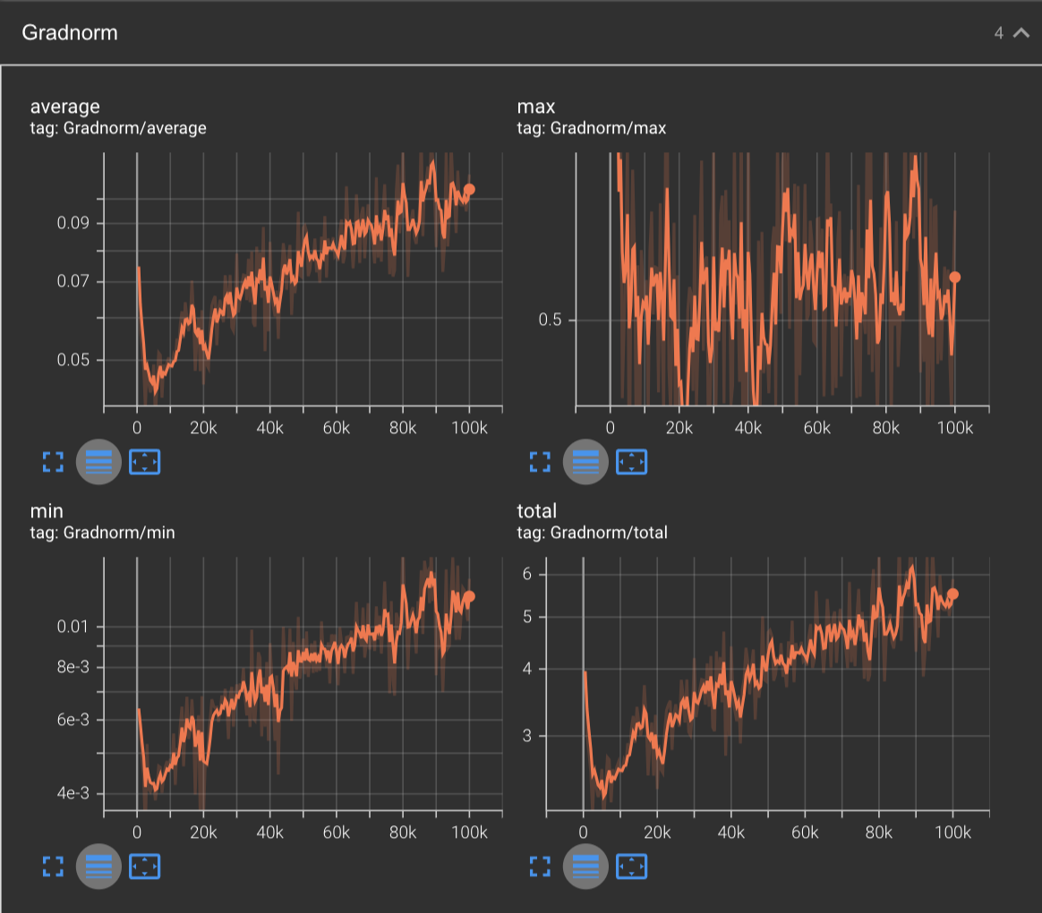
Inspecting the gradnorms with a logarithmic plot, we can see that it is steadily increasing across the board - even the minimum gradnorm is above 0.01, with the total gradnorms across the board adding up to 5.5. This tells us that the gradients are getting greater and greater, indicating a steepening loss landscape.

Moving on from this, let’s check how SGD performs when we set momentum to $0.9$:

SGD with Momentum

Since we’ve consolidated all of our SGD logic into a single class, we can have SGD optimize with momentum by passing the --momentum flag:

python3.11 makemore.py \
  --type='transformer' \
  --learning-rate=1e-3 \
  --optimizer='sgd' \
  --work-dir='out/transformer-nag-momentum-0.9' \
  --max-steps=100000  \
  --momentum=0.9

Just by adding momentum to the optimization process, we can see an instant improvement in our convergence speed:

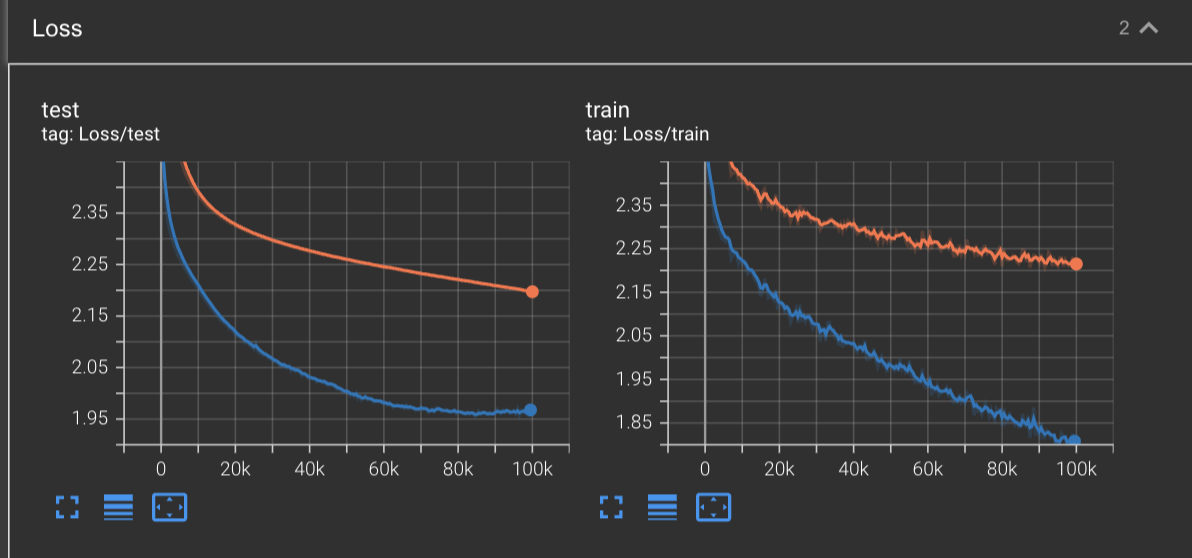
Here we can see the training loss of SGD + momentum (blue) converge down to 1.808, and the test loss all the way down to around 1.968. Here, we’re also starting to see indication of us beginning to overfit on our training data, as it seems like the test curve is beginning to inflect upwards. Compare this to the vanilla SGD results (orange), we have already made a tremendous amount of progress with this simple addition.

We can see a similar story by inspecting the gradnorm:

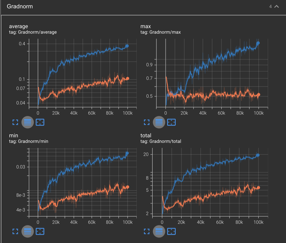
Here we can see that our gradnorm for SGD + momentum (blue) start to increase at an increased rate compared to vanilla SGD (orange).

Nesterov’s Accelerated Gradient

Next, let’s see how this compares with Nesterov’s Accelerated Gradient.

python3.11 makemore.py \
  --type='transformer' \
  --learning-rate=1e-3 \
  --optimizer='sgd' \
  --work-dir='out/transformer-nag-momentum-0.9' \
  --max-steps=100000 \
  --momentum=0.9 \
  --nesterov

Below we have the loss curve of the first 100,000 of training Makemore with Nesterov’s Accelerated Gradient (red) compared against standard SGD (orange) and SGD + Momentum (blue).

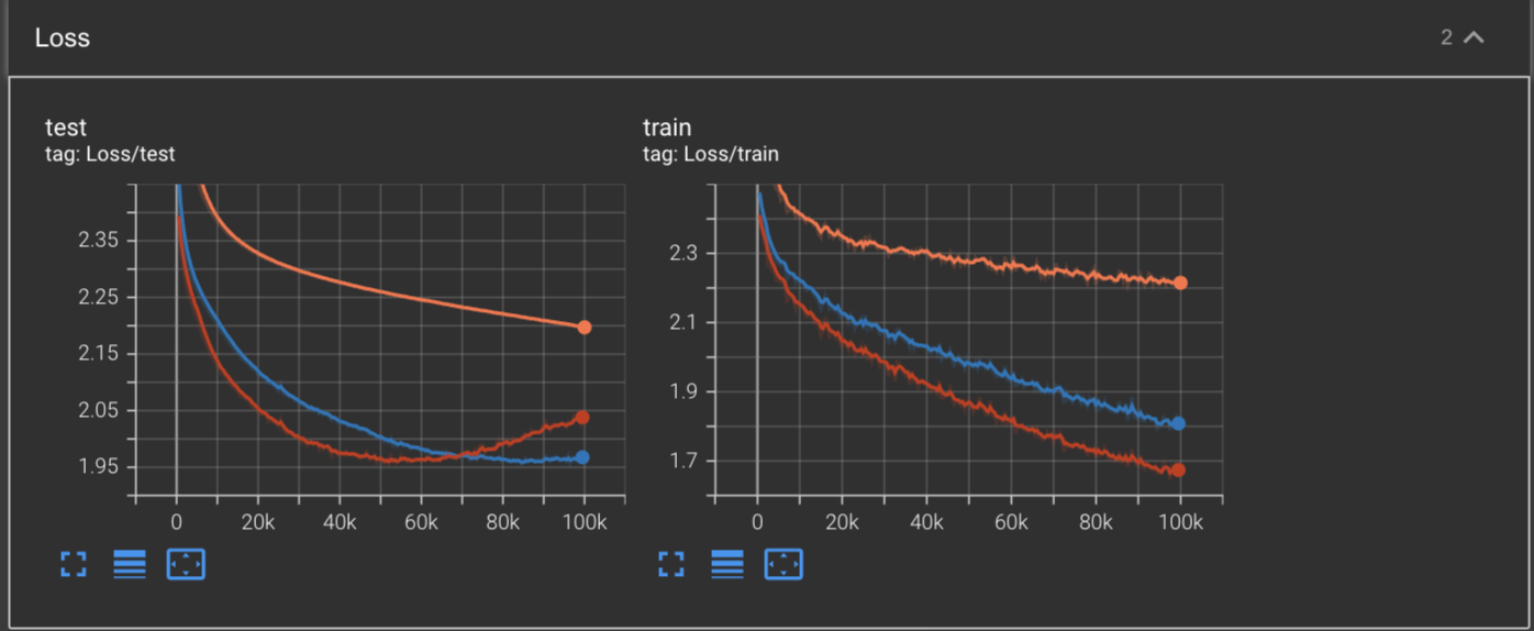
Based on these curves alone, we see that training with NAG causes our network to hit a minimum of a test loss of 1.95 at around 54,000 steps into training. After this, the validation loss begins to climb back up, indicating our network overfitting on the training data.

We also see a new total minimum achieved on the training loss with NAG being the first to reach ~1.67 after training for 100,000 steps.

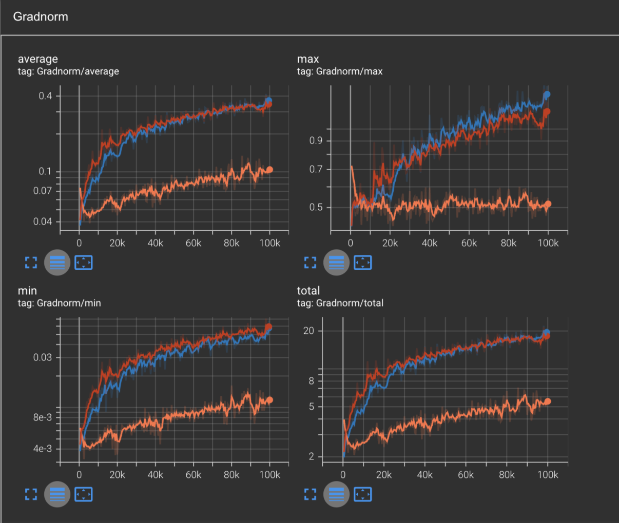
Inspecting the gradnorm shows an interesting result. We see that the actual growth in the gradnorm in NAG (red) doesn’t greatly differ from SGD + momentum (blue). Intuitively this makes sense, since the difference between NAG & regular momentum is simply the point at which we compute the gradient. What’s interesting is how much quicker NAG converges while maintaining a similar gradnorm curve.

Now that we’ve covered convergence on this network and dataset for our first optimizers, let’s move on to the fun part: implementing adaptive optimizers.

The Need for Adaptive Learning-Rate Optimizers

When training deep neural network, our ultimate end goal is to obtain a model which can accurately predict the real world. However; one challenge that we deal with is that we often lack the necessary data to capture all scenarios in which we might be using the model on in the real world.

For example, if we were to build a model which can accurately detect dogs then we’d need to train it on a dataset containing images of dogs. But our dataset might contain images of dogs in conditions where the dogs are looking straight at the camera, appear in good lighting, with a very clear backdrop. But in reality, the model might be seeing the dog from the back, the lighting may be dark, and the backdrop may be cluttered.

For example consider the following two images:

On the left we see an image of a puppy taken under ideal conditions; photos like these are what will comprise our datasets most of time. On the right, we have a photo of a dog in a much more realistic scenario - a dimly lit background, with clutter all over the floor, and an unusual angle at which we view the dog.

As humans, we have the luxury of being able to view these dogs in real-time with spatial information and have enough information to understand exactly what a dog is, what its physical characteristics are, and can use this understanding to identify other dogs down the road.

We are not perfect however; and there may be instances in which we encounter dogs in poor conditions. For instance, if the lights are off and you have a dog that’s sticking its nose in your face or making noise, you might not immediately know what it is. But once we stick our hands out to feel for the dog, we might pick up on the texture of its fur, shape of its body, or its smell to make the connection that this is in fact our dog.

In other words, we are adapting our world knowledge of dogs and how they might appear in situations where our conditions like lighting are suboptimal for instance. But these situations themselves are rare and by the time they arise, we already have a very good idea of what dogs are like in ordinary settings.

In the same way, computers which do not have the luxury of interacting with dogs spatially to build a working knowledge of what they are must also have a mechanism to pick up on these rare features, such as the CCTV footage of the dog above.

One solution to this problem is to use an adaptive learning rate optimizer.

What is an Adaptive Learning-Rate Optimizer?

To understand what an adaptive learning rate optimizer is, we need to understand what SGD is doing. Recall the update rule for SGD:

$${\theta }_{t+1}\leftarrow {\theta }_t-\eta g({\theta }_t)$$

What we’re doing here is saying that - whatever our gradient vector $g({\theta }_t)$ at time $t$ is, make a step of size $\eta$ in the direction towards the function’s minimum.

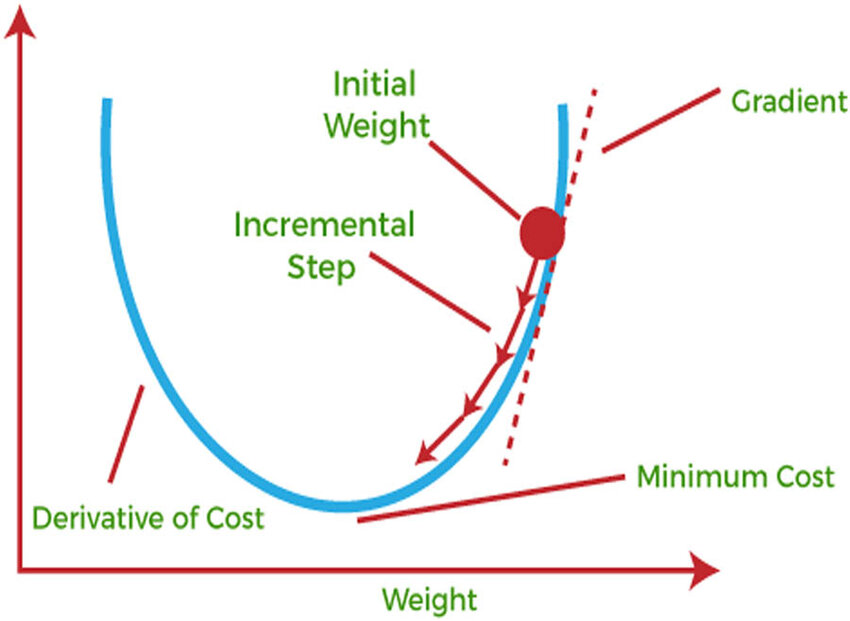
The issue here is that once we begin dealing with a sparse dataset or a complex neural network, we may occasionally encounter rare but important features that the network needs to learn more from than potentially some of the others.

For example, if the network has only seen images of dogs in ideal conditions then it may believe it has a good idea of what dogs looks like. But when it sees a dog in suboptimal conditions, it will be confidently wrong and will therefore need to update its parameters proportionally with the information it just learned.

But notice that under stochastic gradient descent, the only changing variable is the gradient $g({\theta }_t)$ for parameter set ${\theta }_t$. Since the learning rate is constant, we must know the correct setting for it ahead of time. If we set it too high, then we will overshoot our answer and experience oscillations. If we set it too low, then we will experience a slow convergence.

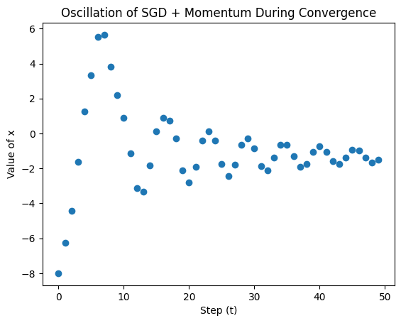
The problem here is that our gradients only tell us the direction of a decreasing loss function, but not how big of a step we should make in that direction.

This is exactly where adaptive learning-rate optimizers come in!

Definition of Adaptive Learning-Rate Optimizers

As the name implies, adaptive learning rate optimizers are optimizers which adjust the learning rate based on some information about the current optimization process.

A few examples of the most well-known adaptive learning-rate optimizers are:

• Adagrad (Adaptive Gradient)
• RMSProp
• Adam
• AdamW

We will cover all of these optimizers in this post.

Adagrad

One of the first widely known adaptive learning-rate optimizers which came to be known is the Adagrad optimizer (short for Adagrad), which was described in the 2011 paper: Adaptive Subgradient Methods for Online Learning and Stochastic Optimization by John Duchi, Elad Hazan, and Yoram Singer.

Adagrad is a parameter-wise adaptive learning-rate optimizer, which means that it adjusts the learning for each parameter independent of the others.

It does this adjustment by following the very simple rule: the more error or noise experienced by a parameter, the smaller its learning rate should be. Intuitively this makes sense, since if a parameter is experiencing a lot of error then it should make smaller fine-grained updates in order to converge to an ideal optimum. On the other hand, if a parameter has been largely stable then it should be open to larger adjustment when the time comes.

Definition

We can represent this relationship quantitatively using the following formula:

$${\eta }_t\leftarrow \eta \cdot \frac{1}{\sqrt{{\sum }_{i=0}^{t}g({\theta }_i{)}^2}+ϵ}$$

Where:

• $\eta$ is the base learning rate that we initial the optimizer with
• ${\eta }_t$ is the learning rate at step $t$
• $g({\theta }_k)$ is the gradient with respect to parameter ${\theta }_k$
• $ϵ$ is a small constant that we use for numerical stability. It’s often set to 1e-8

What Adagrad effectively does is accumulate the squared gradients for each parameter and then scales the learning rate for each parameter by the inverse of the squared root of the accumulated squared gradients.

We therefore represent its update rule by the following:

$$\begin{array}{rl}{G}_0& \leftarrow 0\\ G_t& \leftarrow G_{t-1}+g({\theta }_t{)}^2\\ {\eta }_t& \leftarrow \frac{\eta }{\sqrt{G_t}+ϵ}\\ {\theta }_t& \leftarrow {\theta }_{t-1}-{\eta }_t\cdot g({\theta }_t)\end{array}$$

Where:

• $G_0$ is the initial squared gradient accumulator
• $G_t$ is the accumulated squared gradients at step $t$
• $g({\theta }_t)$ is the gradient at time $t$
• $\eta$ is the base learning rate
• ${\eta }_t$ is the per-parameter scaled learning rate for time $t$
• $ϵ$ is a small constant set for numerical stability

Implementation

The implementation of this optimizer then is very simple. All we must do is accumulate the squared gradients for each parameter, similar to what we had to do when maintaining a per-parameter momentum state.

class Adagrad(Optimizer):
    def __init__(self, params: Iterable[Parameter], lr = 1e-3, eps = 1e-8):
        self.params = [p for p in params]
        self.grad_noise = [torch.zeros_like(p) for p in self.params]
        self.lr = lr
        self.eps = eps

    @torch.no_grad()
    def step(self):
        for i, p in enumerate(self.params):
            # update gradient noise
            self.grad_noise[i] += p.grad.data ** 2
            scaled_lr = self.lr * ((torch.sqrt(self.grad_noise[i]) + self.eps) ** -1)
            p.data = p.data - scaled_lr * p.grad.data

    @torch.no_grad()
    def lr_norms(self) -> List[torch.Tensor]:
        # collect all of the learning rates
        norms = []
        for gn in self.grad_noise:
            norms.append((self.lr * ((torch.sqrt(gn) + self.eps)**-1)).norm(p=2))
        return norms

Notice that our update rule hardly changes from basic SGD. The difference now is that instead of multiplying by self.lr we are instead multiplying by the scaled_lr.

We also introduced a lr_norms method to the optimizer so that we can plot out the L2 norms of the learning rates from within TensorBoard. This will allow us to visualize the non-uniformity of learning rates across different parameters.

Memory consumption:

Adagrad memory consumption: $1\times \text{\# model parameters}$

The Adagrad algorithm consumes $1\times \text{\# model parameters}$ amount of memory. This is because for each model parameter, it needs to store an additional variable for the accumulated squared gradients.

So if you had a 7 billion BF16 parameter model, you would need $42\text{GB}$ to store it, since:

$$\begin{array}{rl}\text{total memory (GB)}& =14\text{ GB (parameters)}+14\text{ GB (gradients)}+14\text{ GB (accumulated squared gradients)}\\ \text{total memory (GB)}& =42\text{ GB}\end{array}$$

Performance During Training

Now that we’ve gotten all of the talk and theory out of the way, let’s see how Adagrad performs in our training scenario!

To run it, we just specify --optimizer=adagrad per our earlier updates:

$ python3.11 makemore.py \
  --type='transformer' \
  --learning-rate=1e-3 \
  --optimizer='adagrad' \
  --work-dir='out/transformer-adagrad' \
  --max-steps=100000

After training the network for 100,000 steps with a base learning rate of 1e-3, we can observe that neither our training loss nor validation loss have effectively converged.

(for the following few analyses, we will omit the SGD data and revisit it at the end of the article)

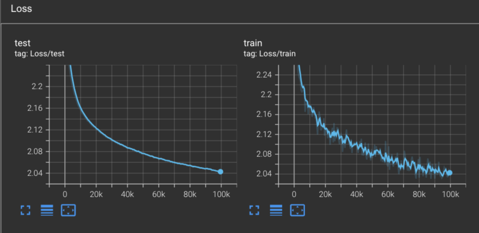
In fact, both the training and test loss are hovering at around 2.043 interestingly enough.

Inspecting the model’s gradnorm over the first 100k steps, we can see that we are far from converged:

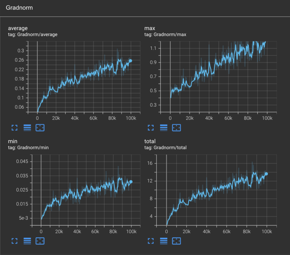
However; an interesting story arises when we plot out the L2 norm of the learning rates. Here we apply TensorBoard’s logarithmic scale for it to be more interpretable:

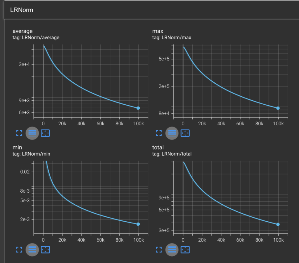
From this graph, we can see a few things: firstly, the learning rate is monotonically decreasing which is exactly what we expect to observe given that our learning rate is scaled by the inverse of accumulated gradients.

Secondly, we can observe that the maximum L2 norm of the learning rates after 100,000 steps is 9.5e4, or $95,000$, whereas the minimum learning rate in our network is ~1.6e-3 or $\approx 0.0016$. Since we know that our learning rate scaling equation, we can solve for this to figure out exactly where this value is coming from:

$$\begin{array}{rl}\Vert {\eta }_t\Vert & =\sqrt{\sum _{i=0}^n{\eta }_{t,i}^2}\\ \Vert {\eta }_t\Vert & =\sqrt{{\eta }^2\sum _{i=0}^n{\left(\frac{1}{\sqrt{G_{t,i}}+ϵ}\right)}^2}\\ \Vert {\eta }_t\Vert & =\eta \sqrt{\sum _{i=0}^n{\left(\frac{1}{\sqrt{G_{t,i}}+ϵ}\right)}^2}\end{array}$$

And thus, plugging in our values for $\Vert {\eta }_t\Vert =95,000$ and $\eta =0.003$, we can get:

$$\begin{array}{rl}95,000& =0.003\sqrt{\sum _{i=0}^n{\left(\frac{1}{\sqrt{G_{t,i}}+ϵ}\right)}^2}\\ 95,000& =\sqrt{\sum _{i=0}^n{\left(\frac{1}{\sqrt{G_{t,i}}+ϵ}\right)}^2}\\ 31,666,666.67& \approx \sqrt{\sum _{i=0}^n{\left(\frac{1}{\sqrt{G_{t,i}}+ϵ}\right)}^2}\\ 1.002777778\times 10^{15}& \approx \sum _{i=0}^n{\left(\frac{1}{\sqrt{G_{t,i}}+ϵ}\right)}^2\end{array}$$

Which can only happen if the combined sum of the inverse accumulated squared gradients is very small. This means that these gradients are coming from parameters which are experiencing very low error rates and are therefore allowed to scale the learning rate up to high values in order to be more open to learning newer features.

But there is one issue with the adaptive gradient optimizer, and it’s that the learning rate is always monotonically decreasing. This means that we rely on our initialization getting us at least somewhat close to the global minimum that we want to optimize towards, or else we may reduce the learning rates prematurely and not converge properly.

To solve this, let’s look at the next optimizer.

RMSProp

The Adagrad optimizer provided a significant breakthrough in the realm of optimizers which adapt the learning rate for each parameter, but it came with the potential issue of the learning rates becoming too low before the network was truly converged.

To get around this, George Hinton proposed Root Mean Square Propogation (RMSProp), an adaptive learning-rate optimizer which uses the moving average of the squared gradient for each parameter, as opposed to the accumulated squared gradients (source: Neural Networks for Machine Learning, Lecture 6a):

$$G_t\leftarrow \alpha G_{t-1}+(1-\alpha )g({\theta }_t{)}^2$$

Where:

• $G_t,G_{t-1}$ are the moving averages from the $t$ and $t-1^{th}$ steps respectively
• $\alpha$ is a used to control the rate of exponential decay of older values
• $g({\theta }_t)$ is the gradient at the $t^{th}$ step

This follows the intuition that if a parameter experience a high gradient / error for a little bit, its learning rate will need to be reduced while we look for its optimum. But once we reach a stable spot, the learning rate should eventually loosen up and allow the parameter to make larger steps again if necessary.

Definition

Thus the full update rule for RMSProp is written as follows:

$$\begin{array}{rl}{G}_0& \leftarrow 0\\ G_t& \leftarrow \alpha \cdot G_{t-1}+(1-\alpha )\cdot g({\theta }_t{)}^2\\ {\eta }_t& \leftarrow \frac{\eta }{\sqrt{G_t}+ϵ}\\ {\theta }_t& \leftarrow {\theta }_{t-1}-{\eta }_t\cdot g({\theta }_t)\end{array}$$

Where:

• $G_0$ is the initial moving average of the squared gradients
• $G_t$ is the moving average of the squared gradients at time $t$
• $\alpha$ is a factor used to control the rate of exponential decay. A common value that works well is $0.99$, though this can be experimented with.
• $g({\theta }_t)$ is the gradient at time $t$
• $\eta$ is the base learning rate
• ${\eta }_t$ is the per-parameter scaled learning rate for time $t$
• $ϵ$ is a small constant set for numerical stability

Though this is the original formulation of RMSprop, there is also a version which incorporates a momentum term. In fact, this is what the PyTorch version actually implements. RMSProp with momentum is simply define as follows:

$$\begin{array}{rl}{G}_0& \leftarrow 0\\ {\mathbf{b}}_0& \leftarrow 0\\ G_t& \leftarrow \alpha \cdot G_{t-1}+(1-\alpha )\cdot g({\theta }_t{)}^2\\ {\mathbf{b}}_t& \leftarrow \mu {\mathbf{b}}_{t-1}+g({\theta }_t)/(\sqrt{G_t}+ϵ)\\ {\theta }_t& \leftarrow {\theta }_{t-1}-{\eta }_t\cdot {\mathbf{b}}_t\end{array}$$

Where:

• ${\mathbf{b}}_0$ is the velocity/buffer at time 0
• ${\mathbf{b}}_t,{\mathbf{b}}_{t-1}$ are the buffers at time $t,t-1$ respectively
• $\mu$ is the momentum factor

If you notice, when we set $\mu =0$ then the above algorithm becomes equivalent to our first definition.

Implementation

Below is the implementation of RMSprop with momentum.

class RMSProp(Optimizer):
    def __init__(self, params: List[Parameter], lr=1e-2, alpha = 0.99, eps = 1e-8, momentum: float = 0):
        self.params = [p for p in params]
        self.variance = [torch.zeros_like(p) for p in self.params] 
        self.velocity = [None for _ in self.params]
        self.lr = lr
        self.alpha = alpha
        self.eps = eps
        self.momentum = momentum

    @torch.no_grad()
    def step(self):
        # very simple optimization step
        for i, p in enumerate(self.params):
            # compute the uncentered variance
            self.variance[i] = self.alpha * self.variance[i] + (1 - self.alpha) * (p.grad.data ** 2)

            if self.momentum > 0:
                # calculation with momentum
                if self.velocity[i] is None:
                    self.velocity[i] = torch.zeros_like(p)

                # here we scale the learning rate with the momentum + rescaled gradient
                scaled_grad = p.grad.data * ((torch.sqrt(self.variance[i]) + self.eps) ** -1)
                self.velocity[i] = self.momentum * self.velocity[i] + scaled_grad

                # now the learning rate gets distributed to both the velocity + scaled gradient
                p.data = p.data - self.lr * self.velocity[i]
            else:
                # simple calculation without momentum
                # step 1: scale the learning rate
                scaled_lr = self.lr * ((torch.sqrt(self.variance[i]) + self.eps) ** -1)

                # step 2: update!
                p.data = p.data - scaled_lr * p.grad.data

    @torch.no_grad()
    def lr_norms(self) -> List[torch.Tensor]:
        norms = []
        for var in self.variance:
            lr = self.lr * ((torch.sqrt(var) + self.eps) ** -1) 
            norms.append(lr.norm(p=2))
        return norms

The above implementation is meant to mirror the PyTorch implementation of RMSprop. However; I was unable to exactly replicate the loss curve produced by the PyTorch RMSprop + momentum implementation, despite having seemingly identical logic.

Memory consumption:

RMSProp memory consumption: $1\times \text{\# model parameters}$

The RMSProp algorithm consumes $1\times \text{\# model parameters}$ amount of memory. This is because for each model parameter, it needs to store an additional variable for the running average of the squared gradients.

So if you had a 7 billion BF16 parameter model, you would need $42\text{GB}$ to store it, since:

$$\begin{array}{rl}\text{total memory (GB)}& =14\text{ GB (parameters)}+14\text{ GB (gradients)}+14\text{ GB (optimizer state)}\\ \text{total memory (GB)}& =42\text{ GB}\end{array}$$

RMSProp + momentum memory consumption: $2\times \text{\# model parameters}$

So if you had a 7 billion BF16 parameter model, you would need $56\text{GB}$ to store it, since:

$$\begin{array}{rl}\text{total memory (GB)}& =14\text{ GB (parameters)}+14\text{ GB (gradients)}+14\text{ GB (squared gradients)}+14\text{ GB (momentum)}\\ \text{total memory (GB)}& =56\text{ GB}\end{array}$$

Performance During Training

Now let’s run the training with our new RMSProp implementation and see what sorts of results we get.

python3.11 makemore.py \
  --type='transformer' \
  --learning-rate=1e-3 \
  --optimizer='rmsprop' \
  --work-dir='out/transformer-rmsprop' \
  --max-steps=100000

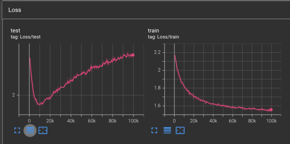
With RMSProp, we achieve the fastest convergence that we’ve seen thus far! After only 10,000 steps, we achieve a test loss minimum of 1.961 before the test results hit an inflection and our network begins to overfit on our training dataset.

And at the end of the 100,000 steps, we achieve a training loss of 1.556. This exceeds the previous record of 1.67 achieved by using Nesterov’s Accelerated Gradient.

If we look at the plot of the learning rate L2 norms, we can see an interesting story arise. Where when we previously trained with Adagrad and saw curves which were strictly decreasing across the board, here we can see that there were actually a few spikes that occurred which caused the learning rates to spike up.

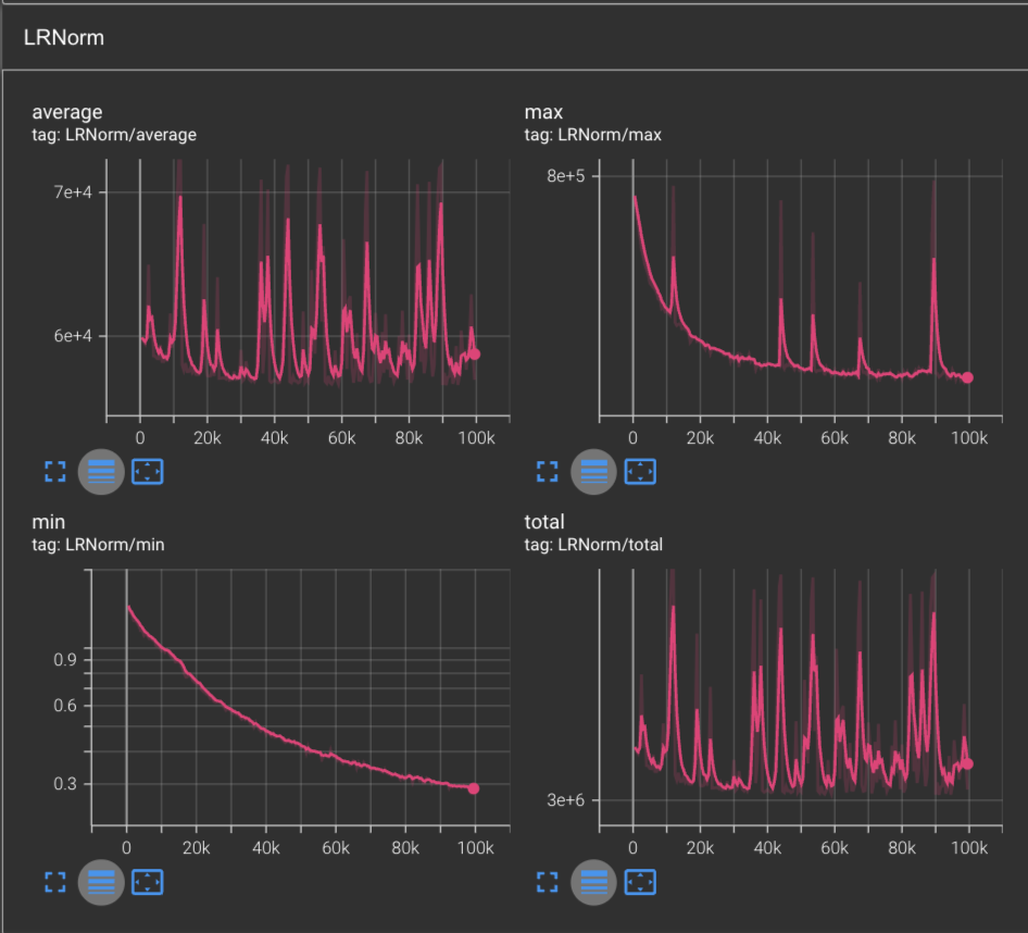
Based on our understanding of RMSProp update step, where we have the scaled learning rate defined by: ${\eta }_t=\frac{\eta }{\sqrt{G_t}+\eta }$ where $G_t=\alpha \cdot G_{t-1}+(1-\alpha )\cdot g({\theta }_t{)}^2$, the only way we could get ${\eta }_t>{\eta }_{t-1}$ is if $\frac{\eta }{\sqrt{G_t}+ϵ}>\frac{\eta }{\sqrt{G_{t-1}}+ϵ}$, which implies that $\sqrt{G_{t-1}}+ϵ>\sqrt{G_t}+ϵ⟹\sqrt{G_{t-1}}>\sqrt{G_t}$ and since we know that $G_t\ge 0\forall t\in \mathbb{Z}$ it follows that $G_{t-1}>G_t$.

Which means that $G_{t-1}>\alpha \cdot G_{t-1}+(1-\alpha )\cdot g({\theta }_t{)}^2$ and we can rewrite this as:

$$\begin{array}{rl}{G}_{t-1}& >\alpha \cdot G_{t-1}+(1-\alpha )\cdot g({\theta }_t{)}^2\\ G_{t-1}-\alpha \cdot G_{t-1}& >(1-\alpha )\cdot g({\theta }_t{)}^2\\ (1-\alpha )\cdot G_{t-1}& >(1-\alpha )\cdot g({\theta }_t{)}^2\\ G_{t-1}& >g({\theta }_t{)}^2\\ \sqrt{G_{t-1}}& >|g({\theta }_t)|\end{array}$$

And therefore we see that the learning rate spikes are in-fact a consequence of the gradients diminishing and thus the optimizer allowing itself to make larger jumps for these parameters.

If we look at the Gradnorm, there is not much of interest, aside from that we see the min & max grandorm curves overall decreasing, while the average hovers at around 0.1 and the total hovers at around 6.

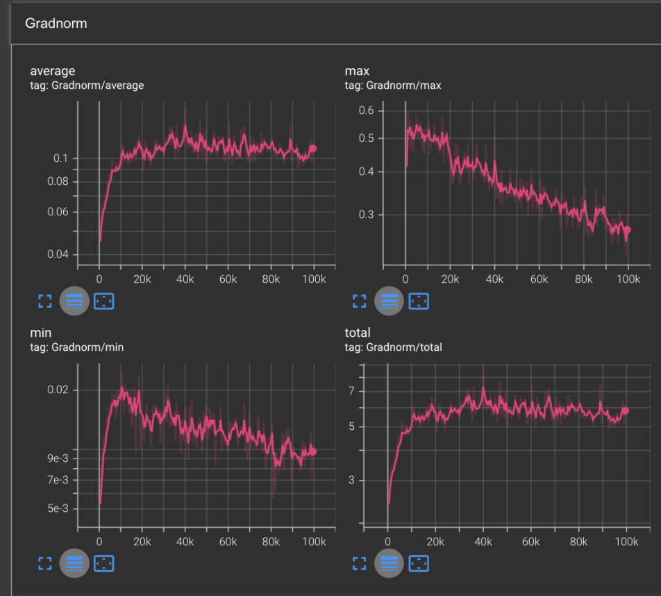
We can infer that some gradients are overall decreasing, while there must be some combinations of gradients within our parameter set that are otherwise adding back to the gradnorm. What’s interesting moreso is that this is the first time we’ve seen an optimizer lead to an overall decrease of gradnorm while training. More interesting yet is that this decrease in the max & min also begins around the 10k step mark.

Bias towards zero

With RMSProp, we seem to have solved the main problem that plagued Adagrad which was the monotonically decreasing learning rates that led us to prematurely kill learning rates before we reached an ideal solution.

However; there is another problem which exists inside of RMSProp that may not be immediately obvious. To understand the issue, let’s consider what happens to RMSProp when we begin to optimize our network from the beginning.

Suppose we set $\alpha =0.99$, a default recommended by PyTorch. Since our sqaured gradients are initialized as $G_0=0$, we compute the optimization step as follows:

$$\begin{array}{rl}{G}_1& \leftarrow 0.99\times 0+0.01\times g({\theta }_1{)}^2\\ G_1& =0.01\times g({\theta }_1{)}^2\\ {\eta }_1& \leftarrow \frac{\eta }{\sqrt{0.01\times g({\theta }_1{)}^2}+ϵ}\\ {\theta }_2& \leftarrow {\theta }_1-\frac{\eta }{\sqrt{0.01\times g({\theta }_1{)}^2}+ϵ}\times g({\theta }_1)\end{array}$$

The issue here is that since we initialize our moving average of the squared gradients to 0, it means that at the beginning of our optimization, this average will be biased towards zero. As a result of this, the learning rate at the beginning may be disproportionately high and will lead us to make large updates even if we may not necessarily want to.

In order to resolve this, let’s look at the Adam optimizer.

Adam

The Adaptive Moment Estimation Optimizer, or Adam for short, is an optimizer that tracks both the momentum as well as the moving average of the squared gradients in order to adaptively scale the learning rates as the error experienced by different parameters fluctuates. Specifically, Adam estimates the first and second moments, and performs a bias correction on both terms before using them in the update rule.

The Adam optimizer was first described in a 2014 paper by Diederik Kingma and Jimmy Ba: Adam: A Method for Stochastic Optimization. Its goal is to provide an effective method for SGD-style optimization but by being able to do both adaptive learning rate scaling as well as leveraging the history of past gradients in order to accelerate the optimization.

How it works

If you understand the concepts presented in RMSProp and SGD + momentum, then Adam is conceptually very similar and easy to understand. We can break it down into the following concepts:

• first moment estimation (momentum)
• second moment estimation (variance)
• bias-corrected moments

At a high level, Adam functions by tracking a quantity known as the first moment estimate and using this as the gradient term in place of where the usual gradient would go when updating the parameters in SGD. It then uses a value called the second moment estimate, just like in RMSProp, to scale the learning rates proportionally for each parameter depending on the amount of error it’s experienced over time.

But rather than using these values exactly, it also corrects each term for the bias towards zero that we saw in RMSProp.

In effect, we can think of the Adam update rule as simply a smarter variant of the vanilla SGD update step. You will see further down that they hold the same form.

First moment estimate

The first moment, or the running average of the gradients, is effectively a quantity that describes the average gradient direction and allows us to smooth out the optimization. We compute the first moment using the following rule:

$$\begin{array}{rl}{m}_0& \leftarrow 0\\ m_t& \leftarrow {\beta }_1\cdot m_{t-1}+(1-{\beta }_1)\cdot g({\theta }_t)\end{array}$$

Where:

• $m_0,m_t$ is the first moment at time $0$ and $t$ respectively
• ${\beta }_1$ is the exponential decay factor for the first moment, and is usually set to ${\beta }_1=0.9$
• $g({\theta }_t)$ is the gradient at time $t$

Conceptually, this is very similar to momentum; however the difference here is that we apply the first moment directly in place of the gradient in the SGD update rule. Where in traditional SGD + momentum we would apply it as:

$$\begin{array}{rl}\overrightarrow{v_t}& \leftarrow \mu {\vec{v}}_{t-1}-\eta g({\theta }_t)\\ {\theta }_{t+1}& \leftarrow {\theta }_t+\overrightarrow{v_t}\end{array}$$

With Adam, we would apply it directly in the update rule:

$$\begin{array}{rl}{m}_t& \leftarrow {\beta }_1\cdot m_{t-1}+(1-{\beta }_1)\cdot g({\theta }_t)\\ {\theta }_{t+1}& \leftarrow {\theta }_t-\eta \cdot m_t\end{array}$$

(note: the update rule above is not the final Adam update rule, it is simply meant to showcase the differences between SGD + momentum and Adam’s first moment estimation)

What the first moment effectively captures is the average of the gradient or the expected gradient.

Second moment estimate

Adam is an adaptive learning-rate optimizer and therefore requires a mechanism to scale the learning rates according to the amount of error being experienced by a given parameter.

To do this, it calculates the second moment estimate. However; there is nothing new about the quantity. In fact, we have already been using it in RMSProp!

The second moment estimate is simply the uncentered variance of the gradients, or in other words: the moving average of the squared gradients! Due to it being uncentered, we also refer to the second moment as the second raw moment of the gradients.

However; in Adam we denote it using $v_t$:

$$\begin{array}{rl}{v}_0& \leftarrow 0\\ v_t& \leftarrow {\beta }_2\cdot v_{t-1}+(1-{\beta }_2)\cdot g({\theta }_t{)}^2\end{array}$$

Where:

• $v_0$ is the second moment estimate at time $t=0$
• $v_{t-1},v_t$ is the second moment estimate at times $t-1$ and $t$ respectively
• ${\beta }_2$ is the exponential decay factor, commonly set to ${\beta }_2=0.999$
• $g({\theta }_t)$ is the gradient at time $t$

Bias correction

As discussed in the section for RMSProp, a key issue of that optimizer was that the initialization of the squared gradient moving average is biased towards 0, since we initialize the average to 0.

To resolve this, the Adam optimizer introduces bias-correction for the first and second moment estimates.

The way this works is that after calculating & updating each estimate, we then compute the bias-corrected estimate terms as follows:

Bias-corrected first moment estimate:

$${\hat{m}}_t\leftarrow \frac{m_t}{1-{\beta }_1^t}$$

Bias-corrected second moment estimate:

$${\hat{v}}_t\leftarrow \frac{v_t}{1-{\beta }_2^t}$$

Bias correction primarily affects the initial steps of optimization, ensuring that the moment estimates are unbiased and providing more accurate updates when $t$ is small.

To illustrate this, let’s view the case when $t=1$:

$$\begin{array}{rl}{m}_1& \leftarrow {\beta }_1\cdot 0+(1-{\beta }_1)\cdot g({\theta }_1)\\ m_1& =(1-{\beta }_1)\cdot g({\theta }_1)\\ {\hat{m}}_1& \leftarrow \frac{(1-{\beta }_1)\cdot g({\theta }_1)}{(1-{\beta }_1)}\\ \therefore {\hat{m}}_1& \leftarrow g({\theta }_1)\end{array}$$

As you can see, by dividng the estimate of the first moment by $(1-{\beta }_1^t)$, this has enabled the first step to simply contain the exact gradient at the first step, as opposed to the gradient scaled by $(1-{\beta }_1)$ (a much smaller number).

However; it’s important to notice that as $t\to \infty$ we get that:

$$\begin{array}{rl}\underset{t\to \infty }{\lim }{\hat{m}}_t& =\underset{t\to \infty }{\lim }\frac{m_t}{(1-{\beta }_1^t)}\\ & =\underset{t\to \infty }{\lim }\frac{m_t}{(1-0)}\\ & =m_t\\ \therefore \underset{t\to \infty }{\lim }{\hat{m}}_t& =m_t\end{array}$$

Which is the exact essence of bias-correction! At the beginning we simply recover the first gradient as necessary, and as time goes on, the bias-correction term simply disappears and we are left with a regular moving average.

The above derivations shown are for the first moment, but they are equally true for the second moment as well.

Update step

Now that we’ve covered the relevant pieces, let’s see how they all come together. In particular, the update step for Adam is defined as:

$${\theta }_{t+1}\leftarrow {\theta }_t-\eta \frac{{\hat{m}}_t}{\sqrt{{\hat{v}}_t}+ϵ}$$

Where:

• ${\theta }_{t+1},{\theta }_t$ are the parameters at time $t+1$ and $t$ respectively
• $\eta$ is the base learning rate, typically initialized to $0.001$
• ${\hat{m}}_t$ is the bias-corrected first moment estimate at time $t$
• ${\hat{v}}_t$ is the bias-corrected second moment estimate at time $t$
• $ϵ$ is a small constant used for numerical stability, typically it is set to 1e-8

We therefore write the full set of update rules for Adam as follows:

$$\begin{array}{rl}{m}_0& \leftarrow 0\\ v_0& \leftarrow 0\\ m_t& \leftarrow {\beta }_1\cdot m_{t-1}+(1-{\beta }_1)\cdot g({\theta }_t)\\ v_t& \leftarrow {\beta }_2\cdot v_{t-1}+(1-{\beta }_2)\cdot g({\theta }_t{)}^2\\ {\hat{m}}_t& \leftarrow \frac{m_t}{1-{\beta }_1^t}\\ {\hat{v}}_t& \leftarrow \frac{v_t}{1-{\beta }_2^t}\\ {\theta }_{t+1}& \leftarrow {\theta }_t-\eta \frac{{\hat{m}}_t}{\sqrt{{\hat{v}}_t}+ϵ}\end{array}$$

As we can see from the above update steps, the overall idea of Adam is very simple. If SGD + momentum is like a hockey puck sliding around on an icy surface, Adam is like a heavy ball that is steadily rolling towards a minima.

Implementation

The implementation of Adam is thus fairly straightforward. We just need to store 2x extra parameters for each model parameter: one for the first moment estimate and another for the second moment estimate.

Here’s the full implementation in Python:

class Adam(Optimizer):
    def __init__(self, params: List[Parameter], lr=1e-3, betas=(0.9, 0.999), eps=1e-8):
        self.lr = lr
        self.eps = eps
        self.params = [p for p in params]
        self.momentum = [torch.zeros_like(p) for p in self.params]
        self.variance = [torch.zeros_like(p) for p in self.params]
        
        # beta values + correction accumulators
        self.b1, self.b2 = betas
        self.b1_accum, self.b2_accum = 1, 1


    @torch.no_grad()
    def step(self):
        # first update the correction accumulators
        self.b1_accum *= self.b1
        self.b2_accum *= self.b2
        for i, p in enumerate(self.params):
            # update moments
            self.momentum[i] = self.b1 * self.momentum[i] + (1 - self.b1) * p.grad.data
            self.variance[i] = self.b2 * self.variance[i] + (1 - self.b2) * (p.grad.data ** 2)

            # correct for bias towards zero
            momentum_c = self.momentum[i] / (1 - self.b1_accum)
            variance_c = self.variance[i] / (1 - self.b2_accum)

            # scale the learning rate & update
            lr = self.lr * ((torch.sqrt(variance_c) + self.eps) ** -1)
            p.data = p.data - lr * momentum_c

    @torch.no_grad()
    def lr_norms(self) -> List[torch.Tensor]:
        assert self.b2_accum != 1, "lr_norms cannot be called before making a step with Adam"
        norms = []
        for var in self.variance:
            corrected = var / (1 - self.b2_accum)
            lr = self.lr * ((torch.sqrt(corrected) + self.eps) ** -1)
            norms.append(lr.norm(p=2))
        return norms

Note: the lr_norms function is strictly for visualization purposes and is not a standard method in PyTorch.

Memory consumption:

Adam memory consumption: $2\times \text{\# model parameters}$

The Adam algorithm consumes $2\times \text{\# model parameters}$ amount of memory. This is because for each model parameter, it needs to store an additional variable for the raw first moment and another variable for the raw second moment.

So if you had a 7 billion BF16 parameter model, you would need $56\text{GB}$ to store it, since:

$$\begin{array}{rl}\text{total memory (GB)}& =14\text{ GB (parameters)}+14\text{ GB (gradients)}+14\text{ GB (first moment)}+14\text{ GB (second moment)}\\ \text{total memory (GB)}& =56\text{ GB}\end{array}$$

Performance during training

Let’s evaluate how well Adam performs in our scenario:

python3.11 makemore.py \
  --type='transformer' \
  --learning-rate=1e-3 \
  --optimizer='adam' \
  --work-dir='out/transformer-adam' \
  --max-steps=100000

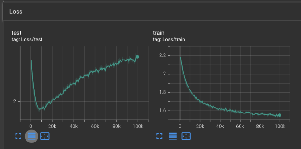
Based on our training data, Adam is the most effective optimizer thus far. It successfully overfits on the training data but at a faster rate than even RMSProp, hitting the validation minima of 1.974 after only 7k steps, a new record! We also hit a new minimum training loss of 1.55 after 100k steps, beating RMSProp’s previous record of 1.556.

The learning rates show an even more interesting story. We see that the learning rates initially all start out high, but taper off much more smoothly. We do hit a few points where we see some minor spikes, but these pale in comparison to the learning rates we saw with RMSProp.

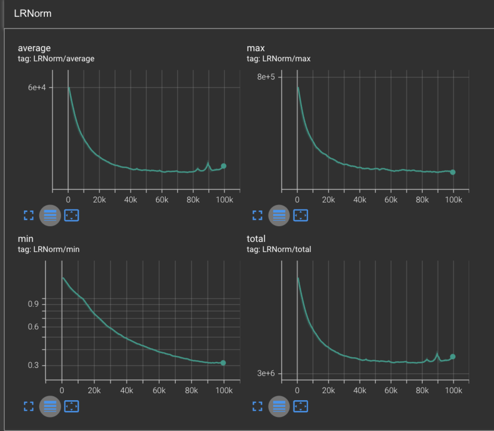
The only curves which don’t drastically change from RMSProp is the gradnorm, where we see similar performance as before. Indicating that the model is doing an overall good job of learning & converging.

Some interesting properties of Adam

Signal-to-noise ratio

One interesting aspect of Adam is that the ratio between the first moment and the square root of the second moment form a signal-to-noise ratio (SNR):

$$\text{SNR}=\frac{{\hat{m}}_t}{\sqrt{{\hat{v}}_t}}$$

The intuition behind the signal-to-noise ratio is as follows:

When ${\hat{m}}_t$ is low but $\sqrt{{\hat{v}}_t}$ is high, we know that particular parameter has experienced high gradients historically, but is unsure about its value for the first moment. Therefore the SNR would be low.

Conversely, if we have that ${\hat{m}}_t$ is high and $\sqrt{{\hat{v}}_t}$ is low, then we interpret this as the parameter experiencing a low amount of error but knowing exactly where it needs to go, and therefore being extremely confident in its convergence.

Then in the cases when ${\hat{m}}_t$ and $\sqrt{{\hat{v}}_t}$ are proportional and roughly equal to each other, then we interpret this as the parameter being confident in its convergence.

We can summarize this relationship with the following table:

${\hat{m}}_t$ \ $\sqrt{{\hat{v}}_t}$	Low	High
Low	Proportionate SNR, high confidence	Low SNR, low confidence
High	Very high SNR, extreme confidence	Proportionate SNR, high confidence

Convergence

Due to how Adam combines the first and second moment estimates for its parameter update step, it’s able to ensure that not only each parameter is able to maintain momentum when being updated, but that the step-size is proportionate to the “bumpiness” of the loss landscape as well.

You can think of it almost as one of those offroad jeeps that have heavy shock absorbers:

In some sense, Adam is very similar in that some wheels (parameters) experience a high amount of change (gradients) and therefore need to be adjusted proportionally (low learning rates) but will not have much room left-over for more rapid elevation changes due to the suspension being compressed, whereas other wheels experience the same momentum but with a low amount of change and therefore will be open to steeper changes in elevation when needed.

Generalization

As an optimizer, Adam is very good at converging down to the nearest minima. However, in some cases, Adam’s ability to adapt learning rates for each parameter can lead to issues with generalization. Conversely, optimizers such as SGD + Momentum and Nesterov’s Accelerated Gradient often exhibit better generalization performance, potentially due to their consistent learning rates across parameters. Nonetheless, the optimal choice of optimizer can depend on the specific task and model architecture.

AdamW

As noted in the previous section, one major drawback of using Adam (as well as other adaptive learning-rate algorithms such as Adagrad & RMSProp) is the poor generalization performance when compared to SGD + momentum.

This is bad news as it particularly affects networks specializing in images or character-level language modeling – which is exactly the goal of Makemore!

Luckily, a paper published in 2017 by Ilya Loshchilov and Frank Hutter, Decoupled Weight Decay Regularization, explores this issue and comes up with a fairly simple solution: for adaptive learning-rate algorithms, the weight decay must be decoupled from the optimization steps taken with respect to the loss function.

Understanding L2 regularization

But what is L2 regularization and why is it such a big problem for the Adam optimizer?

Regularization itself is a method to prevent a model from overfitting on a dataset that works by having some kind of force push back on the model’s weights from arriving at a minimum. It comes in various forms, for instance architectures will often include parameter dropout to randomly kill connections during the training phase.

To that end, ${\mathbf{L}}_2$ regularization, or ridge regularization as it is commonly referred to, accomplishes this by incorporating the squared magnitude of the weights into the loss calculation to prevent them from becoming too large. Having it be the squared magnitude allows it to penalize weights that grow further away. The end result is that we get a lot of small weights.

The way we apply L2 regularization is by updating the the loss function to contain the squared L2 norm of the weights:

$$L_{\text{reg}}({\theta }_t)=L({\theta }_t)+\frac{\lambda }{2}\Vert {\theta }_t{\Vert }_2^2$$

And therefore, when we take the gradient with respect to parameters, it gets transformed as follows:

$$\begin{array}{rl}\frac{\partial L_{\text{reg}}({\theta }_t)}{\partial {\theta }_t}& =\frac{\partial L({\theta }_t)}{\partial {\theta }_t}+\frac{\lambda }{2}\cdot 2\cdot {\theta }_t\\ & =\frac{\partial L({\theta }_t)}{\partial {\theta }_t}+\lambda {\theta }_t\end{array}$$

Which means that our typical SGD update rule that utilizes L2 regularization will go from:

$${\theta }_{t+1}\leftarrow {\theta }_t-\eta g({\theta }_t)$$

To:

$${\theta }_{t+1}\leftarrow {\theta }_t-\eta (g({\theta }_t)+\lambda {\theta }_t)$$

Weight decay vs. L2 regularization

There is yet another regularization technique known as weight decay which has a simple premise: when performing the update step, we simply subtract the weights by the learning rate $\eta$ times and the weight decay factor $\lambda$:

$${\theta }_{t+1}\leftarrow {\theta }_t-\eta g({\theta }_t)-\eta \lambda {\theta }_t$$

But for SGD, this is exactly the same as the above L2 regularization when we distribute the factor of $\eta$ to the terms inside of the parenthesis.

The issue in the Adam algorithm is that if we replace our loss function $L({\theta }_t)$ with the one containing the L2 regularization term $L_{\text{reg}}({\theta }_t)$, it now needs to get injected in 2 different terms: $m_t$ and $v_t$. As a result, the weight decay becomes coupled with the learning rate rescaling that happens in the fraction $\eta \frac{{\hat{m}}_t}{\sqrt{{\hat{v}}_t}+ϵ}$.

How AdamW defines weight decay for adaptive learning-rate algorithms

In order to solve this, AdamW proposes decoupling the weight decay from the loss function. To accomplish this, they simply change the update rule by simply subtracting away the weight decay independent of the learning rate rescaling:

$$\begin{array}{rl}{\theta }_{t+1}& \leftarrow {\theta }_t-\eta \frac{{\hat{m}}_t}{\sqrt{{\hat{v}}_t}+ϵ}-\eta \lambda {\theta }_t\\ {\theta }_{t+1}& \leftarrow {\theta }_t-\eta (\frac{{\hat{m}}_t}{\sqrt{{\hat{v}}_t}+ϵ}+\lambda {\theta }_t)\end{array}$$

Here’s the exact algorithm from the AdamW paper:

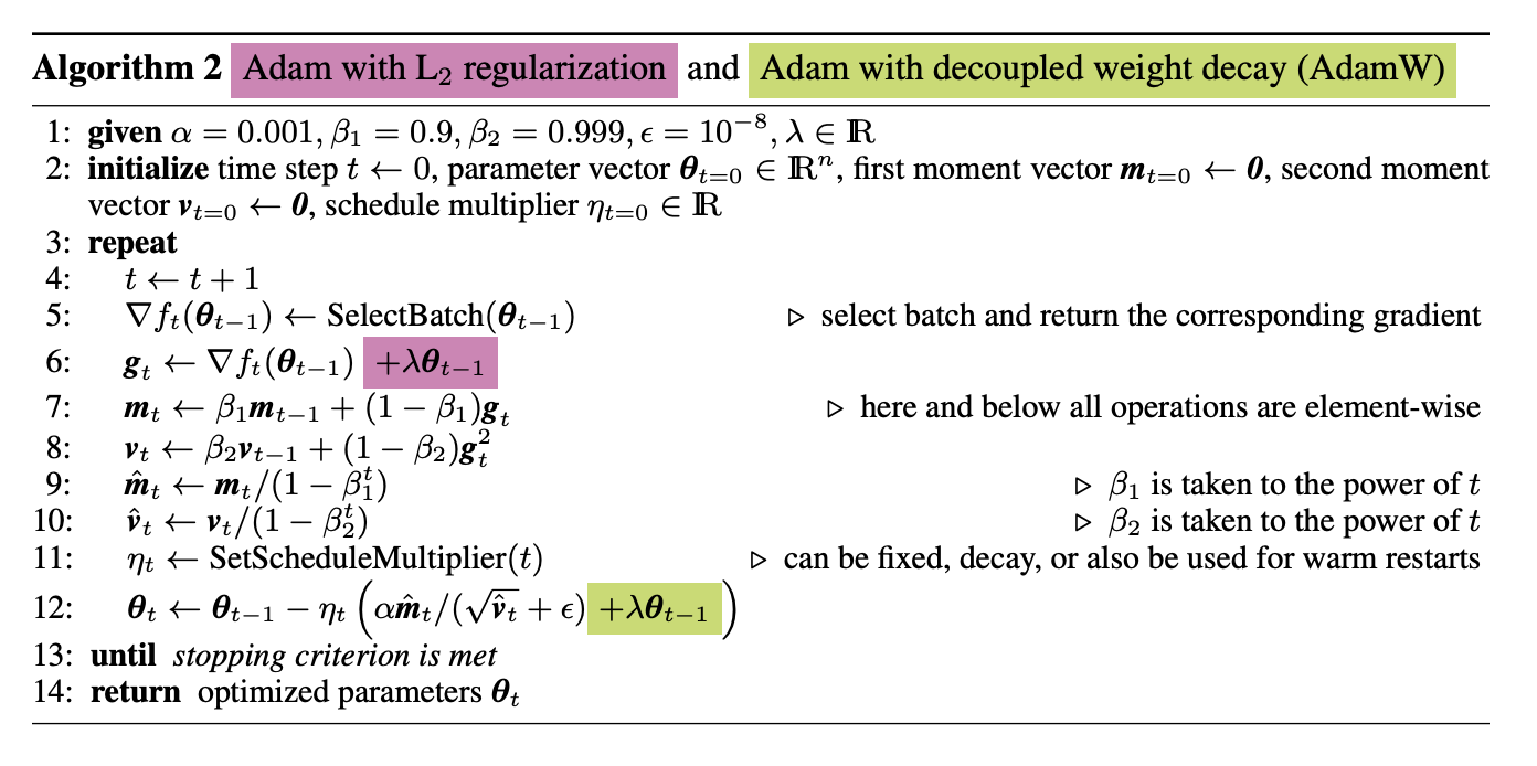
In summary, the challenge Adam faced when originally trying to incorporate weight decay was that it was assumed to be identical to L2 regularization. Ilya Loshchilov and Frank Hutter addressed this issue by decoupling weight decay from L2 regularization and showed that as a result, AdamW was able to generalize much better and achieves comparable results to SGD + Momentum.

However, it’s important to recognize that the generalization performance can vary based on the specific model architecture, dataset, and hyperparameter configurations. Recent advancements and variants like AdamW have aimed to mitigate these issues, offering improved generalization in many scenarios.”

AdamW Update Rule

Since we’ve gone through the differences between Adam and AdamW in the previous section, I will showcase the full update rule here:

$$\begin{array}{rl}{m}_0& \leftarrow 0\\ v_0& \leftarrow 0\\ m_t& \leftarrow {\beta }_1\cdot m_{t-1}+(1-{\beta }_1)\cdot g({\theta }_t)\\ v_t& \leftarrow {\beta }_2\cdot v_{t-1}+(1-{\beta }_2)\cdot g({\theta }_t{)}^2\\ {\hat{m}}_t& \leftarrow \frac{m_t}{1-{\beta }_1^t}\\ {\hat{v}}_t& \leftarrow \frac{v_t}{1-{\beta }_2^t}\\ {\theta }_{t+1}& \leftarrow {\theta }_t-\eta \left(\frac{{\hat{m}}_t}{\sqrt{{\hat{v}}_t}+ϵ}-\lambda {\theta }_t\right)\end{array}$$

Where:

• ${\theta }_{t+1},{\theta }_t$ are the parameters at time $t+1$ and $t$ respectively
• $\eta$ is the base learning rate, typically initialized to $0.001$
• $m_t,v_t$ are the raw first and second moment estimates at time $t$
• ${\beta }_1,{\beta }_2$ are the exponential decay factors for the first & second moment estimates, respectively. They are commonly defaulted to $0.9,0.999$ respectively.
• ${\hat{m}}_t,{\hat{v}}_t$ are the bias-corrected first and second moment estimates at time $t$
• $ϵ$ is a small constant used for numerical stability, typically it is set to 1e-8
• $\lambda$ is the weight decay factor, a common default set here is $\lambda =0.01$.

Implementation

Here’s the full implementation of the AdamW algorithm as it exists in PyTorch:

class AdamW(Optimizer):
    def __init__(self, params: List[Parameter], lr=1e-3, betas=(0.9, 0.999), eps=1e-8, weight_decay=0.01):
        self.lr = lr
        self.eps = eps
        self.weight_decay = weight_decay
        self.params = [p for p in params]
        self.momentum = [torch.zeros_like(p) for p in self.params]
        self.variance = [torch.zeros_like(p) for p in self.params]
        
        # beta values + correction accumulators
        self.b1, self.b2 = betas
        self.b1_accum, self.b2_accum = 1, 1

    @torch.no_grad()
    def step(self):
        # first update the correction accumulators
        self.b1_accum *= self.b1
        self.b2_accum *= self.b2
        for i, p in enumerate(self.params):
            # perform decay
            p.data = p.data - self.lr * self.weight_decay * p.data

            # update moments
            self.momentum[i] = self.b1 * self.momentum[i] + (1 - self.b1) * p.grad.data
            self.variance[i] = self.b2 * self.variance[i] + (1 - self.b2) * (p.grad.data ** 2)

            # correct for bias towards zero
            momentum_c = self.momentum[i] / (1 - self.b1_accum)
            variance_c = self.variance[i] / (1 - self.b2_accum)

            # scale the learning rate & update
            lr = self.lr * ((torch.sqrt(variance_c) + self.eps) ** -1)
            p.data = p.data - lr * momentum_c

    @torch.no_grad()
    def lr_norms(self) -> List[torch.Tensor]:
        assert self.b2_accum != 1, "lr_norms cannot be called before making a step with Adam"
        norms = []
        for var in self.variance:
            corrected = var / (1 - self.b2_accum)
            lr = self.lr * ((torch.sqrt(corrected) + self.eps) ** -1)
            norms.append(lr.norm(p=2))
        return norms

Memory consumption:

AdamW memory consumption: $2\times \text{\# model parameters}$

The AdamW algorithm consumes $2\times \text{\# model parameters}$ amount of memory. This is because for each model parameter, it needs to store an additional variable for the raw first moment and another variable for the raw second moment.

So if you had a 7 billion BF16 parameter model, you would need $56\text{GB}$ to store it, since:

$$\begin{array}{rl}\text{total memory (GB)}& =14\text{ GB (parameters)}+14\text{ GB (gradients)}+14\text{ GB (first moment)}+14\text{ GB (second moment)}\\ \text{total memory (GB)}& =56\text{ GB}\end{array}$$

Performance During Training

Now that we’ve gone through the theory and implementation, let’s see how AdamW performs in practice under our existing examples. As usual, we can run this using:

python3.11 makemore.py \
  --type='transformer' \
  --learning-rate=1e-3 \
  --optimizer='adamw' \
  --work-dir='out/transformer-adamw' \
  --max-steps=100000

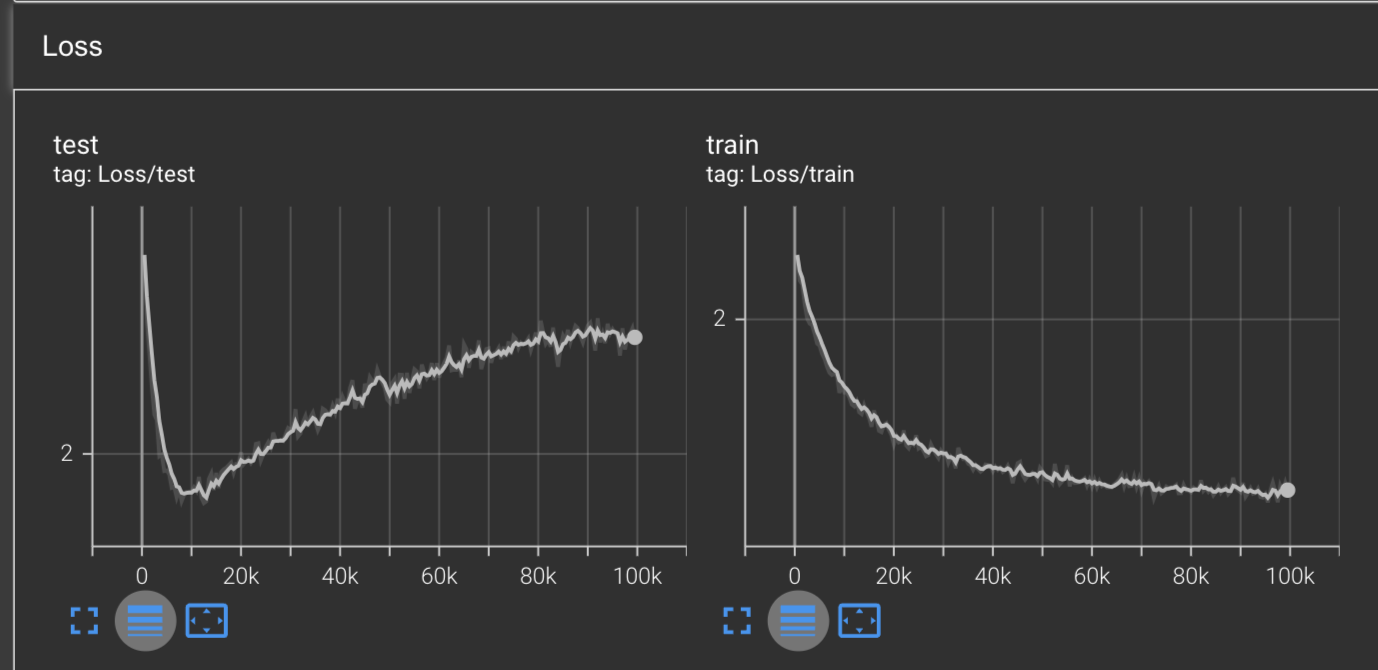
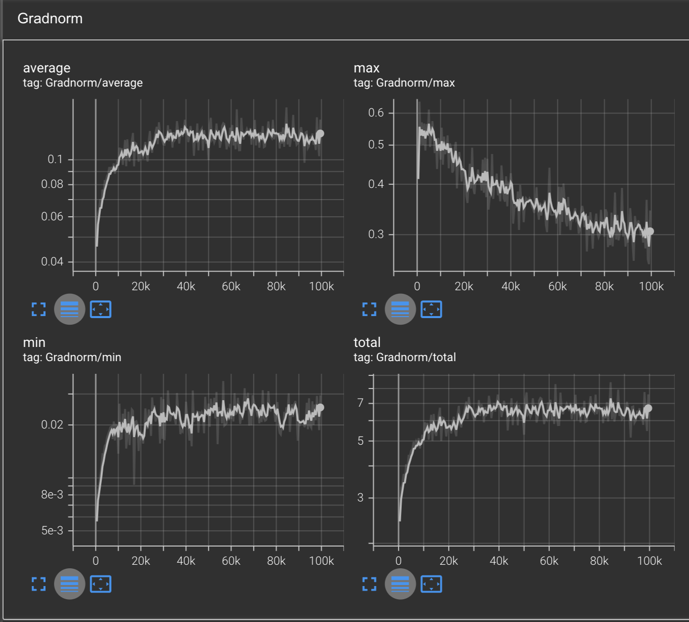
Visually speaking, we appear to get similar results with AdamW as we did with Adam. We reached a global minimum on the training loss of 1.961 at around 9.5k steps. And after 100k steps, we reach a training loss of 1.56, similar to what we hit with Adam and RMSProp.

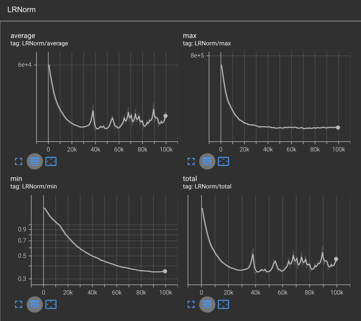
Our LRNorm values are more interesting, where we see no spikes on the min and max LRNorms, but the average and total LRNorms observe a sea of sharp spikes after 30k steps. This is in contrast with our LRNorms for Adam where we saw them be smooth across the board.

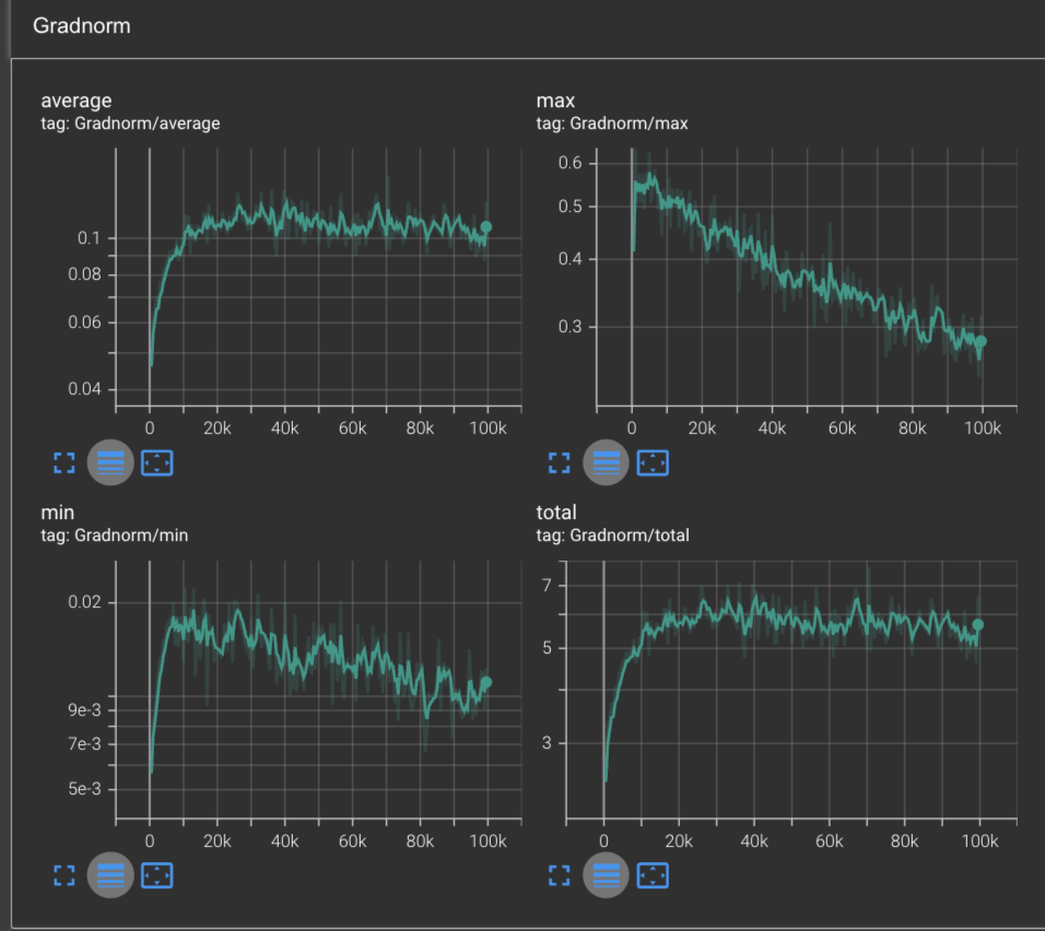
Our gradnorms also look about the same as Adam, except now the min gradnorm is plateuing, where previously both the min and max were decreasing over time.

Final comparisons across all optimizers

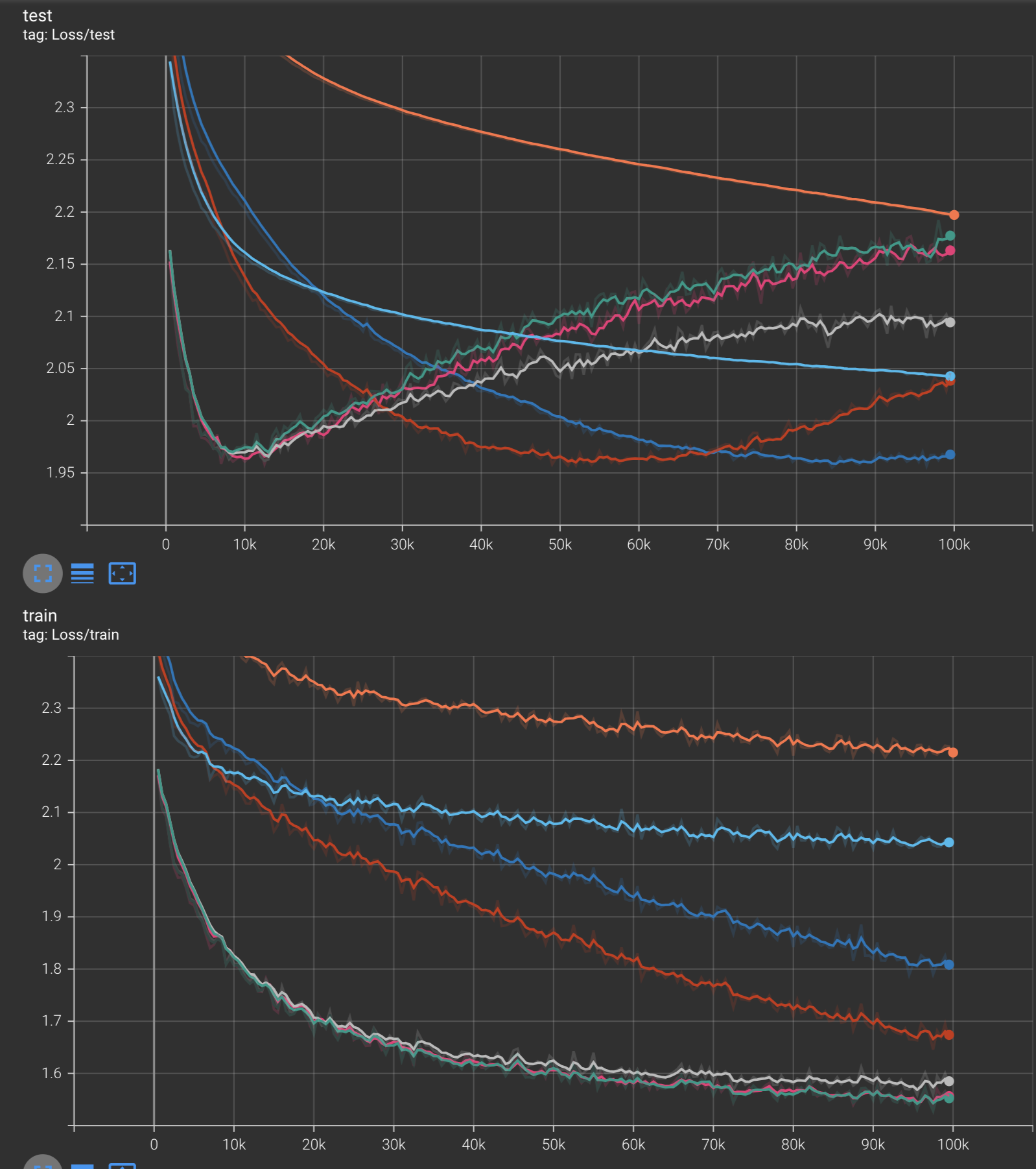
As a final treat for this blog, here are the graphs from all of the optimizers in the training of Makemore.

Training/Test Loss

Optimizer Legend:

Gradnorms

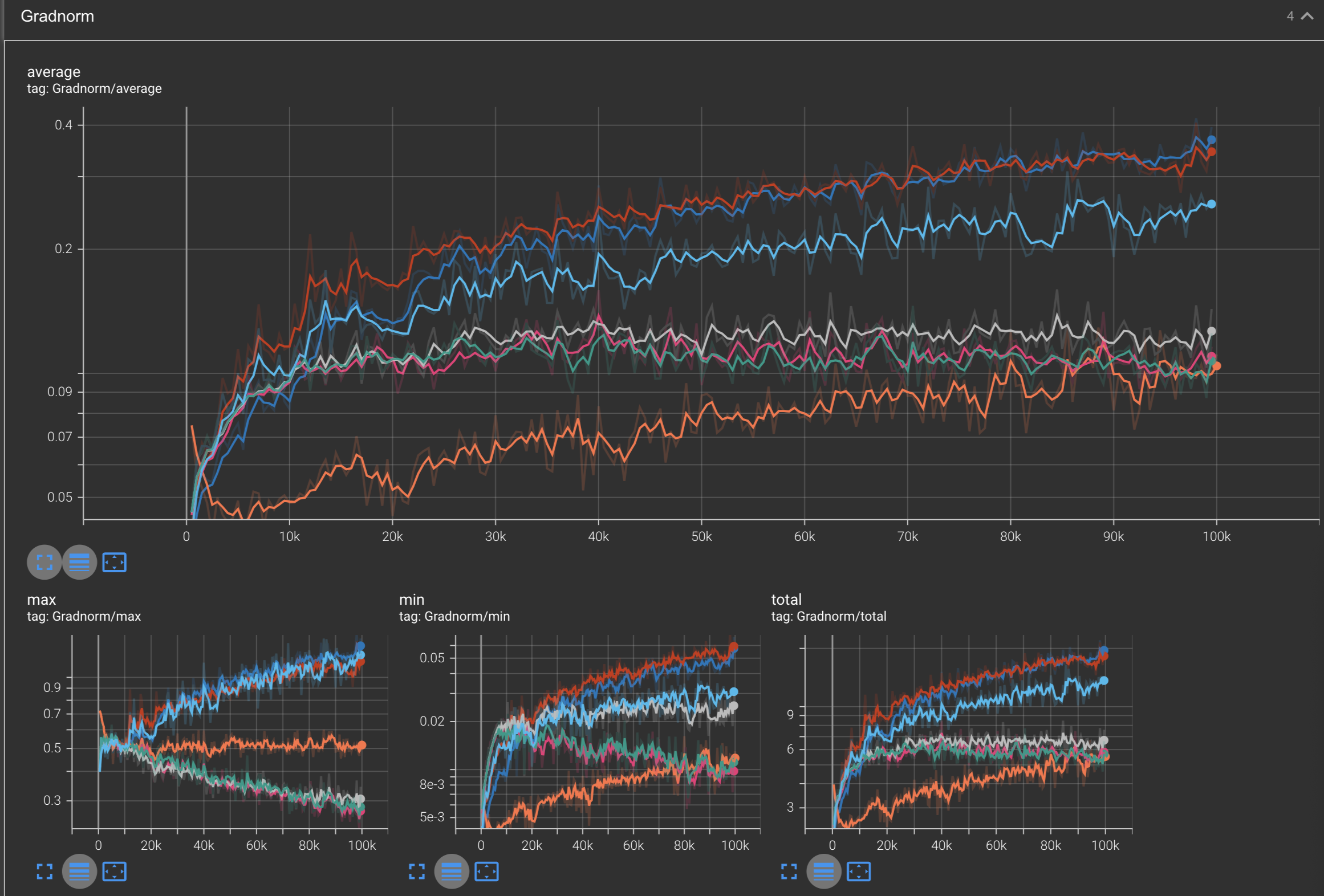
Optimizer Legend:

LRNorms

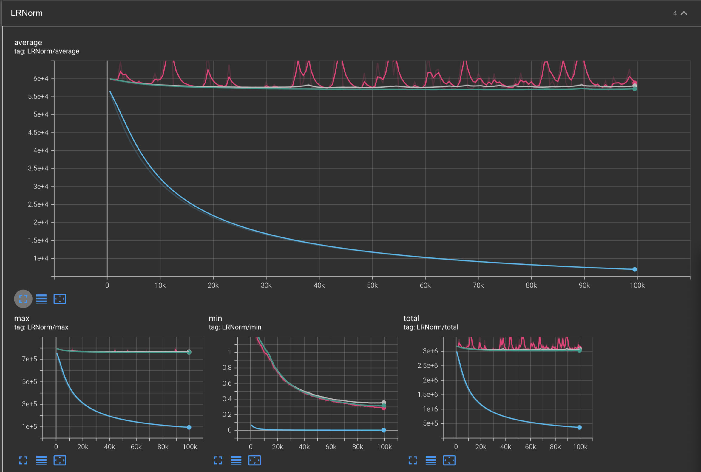
Optimizer Legend:

Conclusion

In summary, we explored how effective optimizers become when they are given the ability to adapt their learning rates for each parameters. We also learned how to derive and implement Adagrad, RMSProp, Adam, and AdamW from scratch in this blog post. We also compared each optimizer against each other when training the Makemore model on Andrej Karpathy’s dataset of names, and saw how some optimizers such as Adam, AdamW, RMSProp, and NAG were able to overfit on the dataset, while some others such as Adagrad had not yet converged after 100k steps of training.

In the next section, we will look at various optimizations that can be made during the training process which are strongly recommended to understand in order to reimplement FSDP from scratch:

• Gradient Accumulation
• Gradient clipping
• Mixed precision training

You can find all of the code that we implemented in this blog in my makemore fork: osilkin98/Makemore.

In addition, I recommend looking into the following resources:

• Previous blog: Momentum-based optimizers from scratch
• Andrej Karpathy’s Makemore repo: karpathy/Makemore
• Neural Networks: Zero to Hero
• Adagrad paper: Adaptive Subgradient Methods for Online Learning and Stochastic Optimization
• George Hinton’s RMSProp lecture: Neural Networks for Machine Learning, Lecture 6a
• Adam paper: Adam: A Method for Stochastic Optimization
• AdamW paper: Decoupled Weight Decay Regularization