From ZeRO to Hero: Rebuilding FSDP From Scratch

Introduction

By the end of this series you will have seen how to implement your own version of FSDP that can perform distributed training. But to do this effectively, we will need to break up the series in order to understand the following foundational concepts:

Foundations of Optimization
Memory Management Techniques in Optimization
Distributed Data Parallelism
Memory Optimization in Distributed Training
Model Parallelism
ZeRO principles
FSDP

In this blog we will cover the foundations of optimization in Deep Learning. By the end of this blog, you will learn about the following optimizers, the intuition behind them, and how to rebuild them from scratch:

Newton’s Method
Stochastic Gradient Descent (SGD)
SGD with Momentum
Nesterov’s Accelerated Gradient (NAG)

Note: This series is inspired by Andrej Karpathy’s Neural Networks: Zero to Hero series. It’s recommended but not required to go through that first as it builds intuition for neural networks in the first place.

Recommended pre-requisites for this series:

To get the most value out of this series, I highly advise the following pre-requisites:

Some Calculus understanding, specifically about derivatives
Python background
Some understanding of neural networks

Optimizers From Scratch

In the world of machine learning and deep learning, we have a variety of different model architectures which all warrant their own techniques for how they actually learn. However; the training loop is the one thing which is largely universal:

""" high-level psuedocode """

model = Model()
optimizer = Optimizer(model.parameters())

for data in dataset:
  optimizer.zero_grad()
  
  # forward-pass
  loss = model(data)
  
  # backward pass
  loss.backward()

  # optimization step
  optimizer.step()

Although some models like Generative Adversarial Networks (GANs) and Reinforcement Learning (RL) models have slight alterations, we ultimately still use some form of the above training loop.

In many modern applications of deep learning, we typically instantiate some optimizer such as AdamW and simply call loss.backward() and optimizer.step(), then sit back and watch the loss curve decrease over time. However; as Andrej Karpathy pointed out in his blog Yes you should understand backprop:

it is easy to fall into the trap of abstracting away the learning process — believing that you can simply stack arbitrary layers together and backprop will “magically make them work” on your data.

While his focus was on the actual backpropagation steps, I’d argue the same is true for optimizers since each comes with its own upsides & drawbacks, so understanding why we’d want to use one over the other will make us into better engineers.

Introduction

Why optimize?

The following section dives into the fundamentals of neural networks and optimization. You may skip this section if you’re just interested in the code.

Before we can build our own optimizers, we must understand what problem they’re solving and why they are so important in training deep neural networks.

If you remember back in Calculus, we were often given a function $f (x) = x^{2}$ and asked to evaluate its minimum. Algebraically this was simple to do, all you’d do is compute its derivative and solve for 0:

f (x) f^{'} (x) f^{'} (x) 2 x x = x^{2} = 2 x = 0 = 0 = 0 power rule now we have to solve for f^{'} (x) = 0 ∴ f has a minimum at 0

And we were often satisfied by this, since it made sense geometrically:

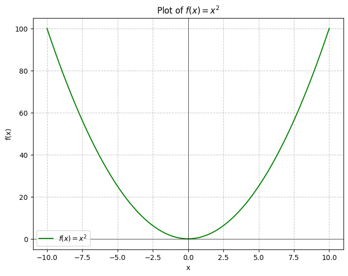
Here we can just look and see that the function is strictly increasing and therefore has a global minimum at $x = 0$ .

But now what if we wanted to find the global minimum of the function $f (x) = sin (x) + \frac{x ^{2}}{10}$ ?:

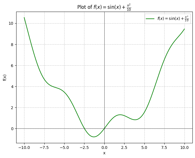
Geometrically we can see that there is clearly a global minimum (in the context of our graph) somewhere around -1, but this isn’t a satisfying enough answer. And what if a slight error here resulted in a rocket landing properly versus crashing into the ocean? We ought to have a better method of finding the answer. Let’s try to do so analytically:

f (x) \frac{df ( x )}{d x} \frac{df ( x )}{d x} = sin (x) + \frac{x ^{2}}{10} = \frac{d}{d x} [sin (x) + \frac{x ^{2}}{10}] = cos (x) + \frac{x}{5}

And then solving for $f^{'} (x) = 0$ :

\frac{df ( x )}{d x} cos (x) + \frac{x}{5} cos (x) x = 0 = 0 = - \frac{x}{5} = cos^{- 1} (- \frac{x}{5})

Well… that’s awkward. We can’t simply find the exact global minimum of this function by solving for $f^{'} (x) = 0$ .

At this point is where we start developing numerical methods which can allow us to find the minimum of the function. One particular method of accomplishing this is Newton’s method.

Newton’s method is a technique which allows us to approximate the roots of a real-valued function by iteratively approaching them using the following formula:

Definition: Newton’s Method

For a differentiable, real-valued function, we can iteratively approximate the roots by computing:
$x_{n + 1} = x_{n} - \frac{f ( x _{n} )}{f ^{'} ( x _{n} )}$

So how can we use this to find the global minimum of our function? Since we’re looking for the global minimum, we can use Newton’s method to find the roots of $f^{'} (x) = 0$ and then simply see which of them is the smallest. We can do this by getting the second derivative of $f (x)$ and plugging them into the equation. In particular, the second derivative is simply: $f^{''} (x) = - sin (x) + 1/5$ . So all we need to do then is compute:

x_{n + 1} = x_{n} - \frac{f ^{'} ( x _{n} )}{f ^{''} ( x _{n} )}

Here’s an implementation of this in Python:

import numpy as np

def fprime2(x):
  # second derivative
  return -np.sin(x) + 0.2

def fprime(x): 
  # first derivative
  return np.cos(x) + x / 5

def f(x):
  return np.sin(x) + (x**2) / 10

def newtons(xi, n):
  x = xi
  for i in range(n):
    fx = f(x)
    fxprime = fprime(x)
    fxprime2 = fprime2(x)
    x = x - (fxprime / fxprime2)
    print(f'[{i:2}/{n:2}] x = {x:.8f}, f(x) = {fx:.5f}, f\'(x) = {fxprime:.5f}, f\'\'(x) = {fxprime2:.5f}')

newtons(-5, 12)

Output:

[ 0/12] x = -5.94388576, f(x) = 3.45892, f'(x) = -0.71634, f''(x) = -0.75892
[ 1/12] x = -7.79433605, f(x) = 3.86580, f'(x) = -0.24579, f''(x) = -0.13283
[ 2/12] x = -6.54310103, f(x) = 5.07695, f'(x) = -1.49926, f''(x) = 1.19822
[ 3/12] x = -5.79428433, f(x) = 4.02422, f'(x) = -0.34221, f''(x) = 0.45700
[ 4/12] x = -6.81783809, f(x) = 3.82703, f'(x) = -0.27601, f''(x) = -0.26966
[ 5/12] x = -6.10875844, f(x) = 4.13875, f'(x) = -0.50312, f''(x) = 0.70954
[ 6/12] x = 2.84660556, f(x) = 3.90524, f'(x) = -0.23693, f''(x) = 0.02646
[ 7/12] x = -1.42425821, f(x) = 1.10104, f'(x) = -0.38748, f''(x) = -0.09073
[ 8/12] x = -1.30751773, f(x) = -0.78643, f'(x) = -0.13884, f''(x) = 1.18928
[ 9/12] x = -1.30644014, f(x) = -0.79458, f'(x) = -0.00126, f''(x) = 1.16554
[10/12] x = -1.30644001, f(x) = -0.79458, f'(x) = -0.00000, f''(x) = 1.16526
[11/12] x = -1.30644001, f(x) = -0.79458, f'(x) = -0.00000, f''(x) = 1.16526

And after 12 iterations, we find that the global minimum of $f (x) = sin (x) + \frac{x ^{2}}{10}$ happens to be around $x \approx - 1.30644$ , which is the same as what WolframAlpha tells us.

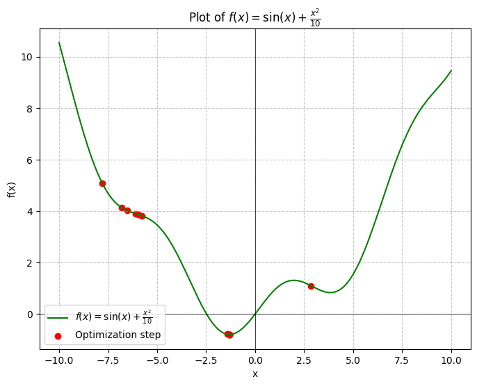
And just like that, we have built our first-ever optimizer from scratch 😃.

Optimization in Machine Learning

Now, what does this have to do with neural networks and deep learning?

Excellent question! In machine learning and deep learning, we typically express a model using a series of differentiable operations such that given an input $x$ and a set of parameters $θ$ , we predict some output value $\overset{y}{^} = f (x; θ)$ . But there’s a problem, how do we know what parameters to use? This is where optimization comes in.

In order to optimize the function $f$ , we need to somehow adjust our parameters such that they yield the desired values. That is, we want to optimize $f$ such that we minimize $∣ y - \overset{y}{^} ∣ = ∣ y - f (x; θ) ∣$ . So how do we do this?

The answer is using loss functions. Specifically, we mathematically define the error in a model’s prediction $L (θ)$ using a differentiable function, and then we calculate the derivative of the function with respect to the model’s parameters. We call this the gradient $g (θ)$ :

Definition: Loss function

A loss function (sometimes called a cost function) is a mathematical method that describes the amount of error in a model’s prediction.

g (θ) = \frac{\partial L}{\partial θ}

(Though it’s usually more succinct to use the nabla character: $g (θ) = \nabla L (θ)$ )

By knowing the gradient of the loss function with respect to a model’s parameters, we therefore know how much the model improves or worsens with respect to some small change in its parameters. Using this information then, we can therefore adjust the gradients in the direction of a decreased loss.

That is — if $g (θ)$ tells us how much the loss increases if we adjusted the parameters by a tiny amount, then $- g (θ)$ is how much the loss decreases when we move the parameters in the opposite direction.

Loss Functions: How do they work?

In order to optimize a model of any kind, we must first define what it is exactly that we’re optimizing. That is, we define the loss/cost function. The purpose of the loss function is to perform the comparison between a model’s prediction and the true value, and output a value which describes how close or far the model was from obtaining the correct answer.

Loss functions themselves can come in many formats, but for ML and DL, they must importantly be differentiable on the entire domain of possible values for a given problem.

The choice of loss function may actually vary depending on the problem you’re dealing with, and there are various scenarios in which many different loss functions may actually do the job. For the sake of this blog we will not be exploring these, but an interesting topic to study are the different loss functions that exist for linear regression such as Mean Squared Error (MSE), Mean Absolute Error (MAE), and Huber Loss. Investigating these may be worth a blog in itself.

Example: Linear Regression

For the sake of example, let’s begin with a simple linear regression example. Let’s suppose we have the set of generated data:

np.random.seed(0)
x = 2 * np.random.rand(100, 1)
y = 4 + 3 * x + np.random.randn(100, 1)
plt.scatter(x, y)
plt.title("Randomly generated data with Numpy seed 0")
plt.xlabel('x')
plt.ylabel('y')

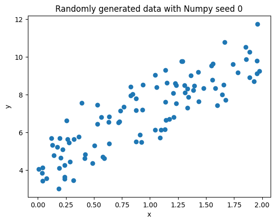
We know that a simple linear regression can be modeled as follows:

f (x; θ) = θ_{1} x + θ_{2}

And we know that outputs are $\overset{y}{^} = f (x; θ)$ .

Let’s therefore initialize a set of parameters to some random values and see how well they plot in this curve.

Click to view the code

np.random.seed(0)
x = 2 * np.random.rand(100, 1)
y = 4 + 3 * x + np.random.randn(100, 1)


# adjust these params for sake of example
p1 = np.random.randn() * 12
p2 = np.random.randn() * -9

x_range = np.arange(0, 2.1, 0.1)
y_range = x_range * p1 + p2


plt.scatter(x, y, label="random data points")
plt.plot(x_range, y_range, label=fr"y = {p1:.2f}x + {p2:.2f}", color='red')


plt.legend()

plt.title("Randomly generated data with Numpy seed 0")
plt.xlabel('x')
plt.ylabel('y')

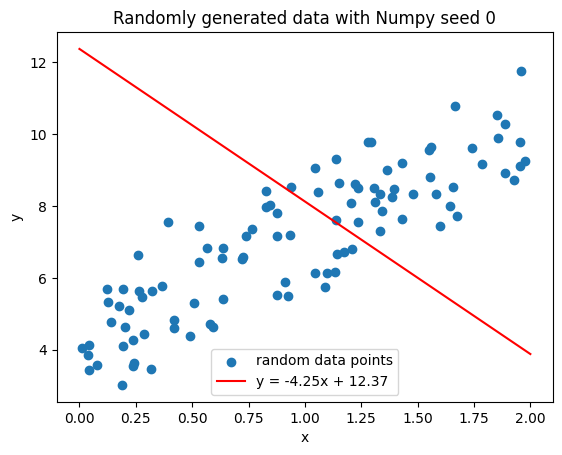
Okay well obviously this is pretty bad, but how can we quantify how bad this is?

To do this, we will make use of Mean Squared Error (MSE):

L (θ) = \frac{1}{n} i = 1 \sum n (y_{i} - \overset{y_{i}}{^})^{2}

Implementing this, we get the following:

# MSE prediction
MSE = (1/x.shape[0]) * ((y - (x * p1 + p2)) ** 2).sum()
MSE
>>> np.float64(20.0717103178283)

Now comes the fun part: using the MSE, how can we optimize the function?

Well it turns out it’s pretty simple. We can take the gradient of the loss and simply go in the opposite direction of the gradient. This process is called gradient descent.

The formula for gradient descent is as follows:

θ_{t + 1} \leftarrow θ_{t} - η g (θ_{t})

Where:

$θ_{t}$ is an arbitrary parameter at timestep $t$ , and $θ_{t + 1}$ is the updated parameter at the following timestep
$η$ is the step size, also known as the learning rate
$g (θ_{t})$ is the derivative of the loss at time $t$ with respect to the given parameter

Note, not denoted in the above formula, but $θ_{t}$ is referring to any particular parameter at a timestep $t$ , the index of which is implicit. In the context of our linear regression example, we would have $θ_{t, i}$ to denote the parameter $i$ at time $t$ .

So to compute the gradient descent for our linear regression example, we will take the gradient for each parameter $θ_{1}$ (slope):

\frac{\partial L}{\partial θ _{1}} = \frac{1}{n} i = 0 \sum n \frac{\partial}{\partial θ _{1}} (y_{i} - \overset{y_{i}}{^})^{2} = \frac{1}{n} i = 0 \sum n 2 (y_{i} - \overset{y_{i}}{^}) \cdot (- \frac{\partial y _{i} ^}{\partial θ _{1}}) = - \frac{1}{n} i = 0 \sum n 2 (y_{i} - \overset{y_{i}}{^}) \cdot \frac{\partial}{\partial θ _{1}} [θ_{1} x + θ_{2}] = - \frac{1}{n} i = 0 \sum n 2 (y_{i} - \overset{y_{i}}{^}) \cdot x

And similarly for $θ_{2}$ (our y-intercept):

\frac{\partial L}{\partial θ _{2}} = \frac{1}{n} i = 0 \sum n \frac{\partial}{\partial θ _{2}} (y_{i} - \overset{y_{i}}{^})^{2} = \frac{1}{n} i = 0 \sum n 2 (y_{i} - \overset{y_{i}}{^}) \cdot (- \frac{\partial y _{i} ^}{\partial θ _{2}}) = - \frac{1}{n} i = 0 \sum n 2 (y_{i} - \overset{y_{i}}{^}) \cdot \frac{\partial}{\partial θ _{2}} [θ_{1} x + θ_{2}] = - \frac{1}{n} i = 0 \sum n 2 (y_{i} - \overset{y_{i}}{^}) \cdot 1 = - \frac{1}{n} i = 0 \sum n 2 (y_{i} - \overset{y_{i}}{^})

Now given these two formulas, let’s write the gradient descent for our linear regression!

# compute loss
MSE = (1/x.shape[0]) * ((y - (x * p1 + p2)) ** 2).sum()
print(f'loss: {MSE.item():.4f}')

# compute derivatives
dp1 = -(2/x.shape[0])  * ((y - (x * p1 + p2)) * x).sum()
dp2 = -(2/x.shape[0]) * (y - (x * p1 + p2)).sum()
print(f'dp1 = {dp1:.4f}, dp2 = {dp2:.4f}')

>>> loss: 20.0717
>>> dp1 = -2.2857, dp2 = 2.6574

We can see in the above step that we have a MSE loss of $20.0717$ , and we also see that we have some values for the derivatives of the loss with respect to either parameter. Now let’s use this information to optimize the linear regression.

In this optimization we use $η = 0.05$ .

# initialize the network
np.random.seed(0)
x = 2 * np.random.rand(100, 1)
y = 4 + 3 * x + np.random.randn(100, 1)

# adjust these params for sake of example
p1 = np.random.randn() * 12
p2 = np.random.randn() * -9

# data 
gradnormsi = []
lossi = []

# training loop
max_iters = 1000
lr = 0.05
for i in range(max_iters):

  # predict step
  y_pred = x * p1 + p2

  # compute loss using mean squared error
  MSE = (1/x.shape[0]) * ((y - y_pred) ** 2).sum()
  
  # compute derivatives
  dp1 = - (2/x.shape[0])  * ((y - y_pred) * x).sum()
  dp2 = - (2/x.shape[0]) * (y - y_pred).sum()

  # backpropagate
  p1 = p1 - lr * dp1
  p2 = p2 - lr * dp2  # Corrected to use dp2 for updating p2

  if i % 50 == 0:
    print(f'[{i:3}/{max_iters:3}] loss: {MSE.item():.4f}')
  
  lossi.append(MSE)
  gradnormsi.append((dp1 ** 2 + dp2 ** 2) ** 0.5)

For which we get the following output:

[  0/1000] loss: 20.0717
[ 50/1000] loss: 4.7583
[100/1000] loss: 1.7357
[150/1000] loss: 1.1392
[200/1000] loss: 1.0214
[250/1000] loss: 0.9982
[300/1000] loss: 0.9936
[350/1000] loss: 0.9927
[400/1000] loss: 0.9925
[450/1000] loss: 0.9924
[500/1000] loss: 0.9924
[550/1000] loss: 0.9924
[600/1000] loss: 0.9924
[650/1000] loss: 0.9924
[700/1000] loss: 0.9924
[750/1000] loss: 0.9924
[800/1000] loss: 0.9924
[850/1000] loss: 0.9924
[900/1000] loss: 0.9924
[950/1000] loss: 0.9924

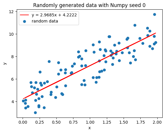
And we see that the model has converged after around 500 steps. If we print out the gradients now, we get the following values:

print(dp1, dp2)

>>> -2.1220866065416611e-07 2.3915423344789135e-07

Let’s see what the plotted line looks like now:

Analyzing Convergence

One question to think about before we move away from the linear regression example: how do we know when we’re done training?

For example, here is the loss curve of the above optimization:

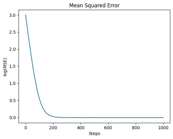
It’s easy to look at the loss curve over time and see that it’s become relatively flat and therefore we’ve reached a minimum. But this isn’t any better than earlier when we were guesstimating the minimum of $f (x) = s in (x) + x^{2} /10$ .

One way to analyze convergence is to inspect the gradnorm, that is, the value of the equation:

∥\nabla∥ = \frac{\partial L}{\partial θ _{1}}^{2} + \frac{\partial L}{\partial θ _{2}}^{2}

What this tells us is the magnitude of the gradient, or effectively its absolute length. The further the gradnorm is from 0, the further we are from an optima.

But If we plot out the log of the gradnorm, we find that we are still converging:

We use the log of the gradnorm to get a better idea of how far away it is from 0.

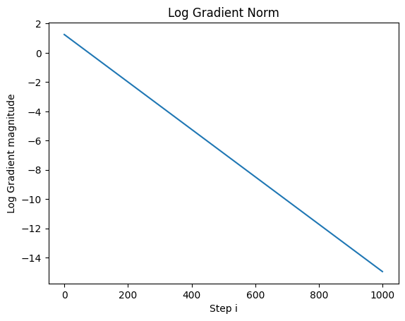
So let’s now run the optimization for 50,000 steps and plot out the gradnorm:

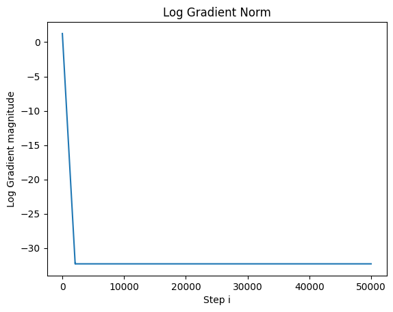
We see now that we have finally converged.

Finally before we move on, let’s compare our approximated values that we got using backpropagation to the calculated values by solving the linear regression:

# Solve the linear regression using numpy's least squares method
A = np.hstack([x, np.ones((x.shape[0], 1))])  # Add a column of ones for the intercept
theta_optimal, _, _, _ = np.linalg.lstsq(A, y, rcond=None)

# Extract the optimal values for the slope and intercept
optimal_slope = theta_optimal[0][0]
optimal_intercept = theta_optimal[1][0]

# Print the optimal values
print(f'Optimal slope (theta_1): {optimal_slope}')
print(f'Optimal intercept (theta_2): {optimal_intercept}')
print(f'Difference between calculated vs. approximated slope: {abs(p1 - optimal_slope)}')
print(f'Difference between calculated vs. approximated intercept: {abs(p2 - optimal_intercept)}')

>>> Optimal slope (theta_1): 2.968467510701021
>>> Optimal intercept (theta_2): 4.222151077447227
>>> Difference between calculated vs. approximated slope: 1.9984014443252818e-14
>>> Difference between calculated vs. approximated intercept: 2.398081733190338e-14

As we see, they are not exact, but if we’re within 1e-14th of each other, at that point it just comes down to floating-point precision errors.

Gradient Descent

Gradient Descent is the simplest form of optimization algorithm. It is when we are able to process the gradient for the entire dataset in a single step, and are therefore making no approximations as to where the gradient could be. We are in essence, taking the true gradient for the set of parameters $θ$ .

However; the issue with Gradient Descent is that it requires us to compute the gradient over the entire dataset (full-batch), when this may not always be feasible to do. For instance, you may have a transformer model for which a single sample being passed through will result in gigabytes of storage being allocated. For this reason, we instead use Stochastic Gradient Descent.

Stochastic Gradient Descent

Stochastic Gradient Descent (SGD) is the simplest optimization algorithm in use for training neural networks. Where in Gradient Descent we computed the gradient for the entire dataset, in SGD we take a mini-batch of samples and compute the average loss across the batch, then compute the gradient.

g (θ_{t}) \leftarrow \frac{1}{B} i = 1 \sum B \nabla L (x_{i}; θ_{t}) θ_{t + 1} \leftarrow θ_{t} - η g (θ_{t})

Where:

$B$ is the batch size
$η$ is the learning rate
$θ_{t}, θ_{t + 1}$ is the parameters set at times $t$ and $t + 1$ respectively
$\nabla L (θ_{t})$ is the gradient of the loss for a single sample $i$ in batch $B$
$g (θ_{t})$ is the gradient averaged across the batch

The algorithm for SGD is as follows:

lr = 0.1
while not_converged:
  # forward pass
  # ...
  # optimize!
  param = param.data - lr * param.grad

Here’s the implementation:

from typing import List
from torch.nn import Parameter
import torch

class StochasticGradientDescent:
  def __init__(self, params: List[Parameter], lr=1e-1):
    self.params = [p for p in params]
    self.lr = lr

  def zero_grad(self, set_to_none=True):
    # we respect `set_to_none` for pytorch compatability
    for p in self.params:
      if set_to_none:
        p.grad = None
      else:
        p.grad.data = torch.zeros_like(p.data)

  @torch.no_grad()
  def step(self):
    # very simple optimization step
    for p in self.params:
      p.data = p.data - self.lr * p.grad.data

We observe that the SGD algorithm is actually quite simpler than using Newton’s method as we did earlier, since we aren’t having to compute the second-order derivative (also referred to as the Hessian matrix) in order to optimize. This can be very beneficial for large models where you have to store both derivatives but also compute the second derivative.

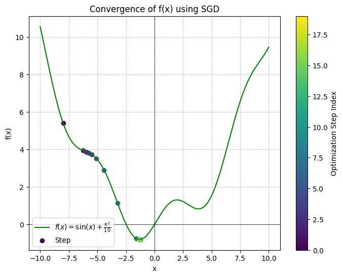
Let’s look at the problem from earlier to see how SGD will find the minimum of our function $f (x) = s in (x) + x^{2} /10$ :

To simulate this convergence, we’ll simply define everything using torch constructs in order to leverage its autograd engine:

import torch
torch.manual_seed(42)

# define our function
def f(x) -> torch.Tensor:
  return torch.sin(x) + (x**2)/10

learning_rate = 1.0
x = torch.tensor([-8], requires_grad=True, dtype=torch.float32)
optimizer = StochasticGradientDescent([x], lr=learning_rate)

# allows us to gauge how close we are to the answer
actual_answer = torch.tensor([-1.30644])
tolerance = 1e-6

N = 20
xs, ys = [], []
for i in range(N):
  optimizer.zero_grad()
  y = f(x)
  xs.append(x.detach().item())
  ys.append(y.detach().item())
  
  # computes dy/dx
  y.backward()
  with torch.no_grad():
    dx = torch.cos(x) + x/5
    if i % 1 == 0:
      print(f'x: {x.item():.4f}, y: {y.item():.4f}, dy/dx: {x.grad.data.item():.4f}, manual dy/dx: {dx.item():.4f}')

    if (diff := abs(x - actual_answer)) <= tolerance:
      break

  
  # performs the optimization
  optimizer.step()


with torch.no_grad():
  print(f"Diff: {diff.item():.5f}, x: {x.item():.5f}, f(x): {f(x).item():.5f}, optimum: {actual_answer.item():.5f}, f(optimum): {f(actual_answer).item():.5f}")
  if (diff := abs(x - actual_answer)) <= tolerance:
    print(f"We've converged after {i} steps!")
  else:
    print(f"We failed to converge after {N} steps!")

Running this, we get the following output:

x: -8.0000, y: 5.4106, dy/dx: -1.7455, manual dy/dx: -1.7455
x: -6.2545, y: 3.9406, dy/dx: -0.2513, manual dy/dx: -0.2513
x: -6.0032, y: 3.8802, dy/dx: -0.2396, manual dy/dx: -0.2396
x: -5.7636, y: 3.8184, dy/dx: -0.2847, manual dy/dx: -0.2847
x: -5.4789, y: 3.7222, dy/dx: -0.4021, manual dy/dx: -0.4021
x: -5.0768, y: 3.5117, dy/dx: -0.6590, manual dy/dx: -0.6590
x: -4.4178, y: 2.9086, dy/dx: -1.1739, manual dy/dx: -1.1739
x: -3.2439, y: 1.1544, dy/dx: -1.6435, manual dy/dx: -1.6435
x: -1.6003, y: -0.7435, dy/dx: -0.3496, manual dy/dx: -0.3496
x: -1.2507, y: -0.7928, dy/dx: 0.0645, manual dy/dx: 0.0645
x: -1.3152, y: -0.7945, dy/dx: -0.0102, manual dy/dx: -0.0102
x: -1.3050, y: -0.7946, dy/dx: 0.0017, manual dy/dx: 0.0017
x: -1.3067, y: -0.7946, dy/dx: -0.0003, manual dy/dx: -0.0003
x: -1.3064, y: -0.7946, dy/dx: 0.0000, manual dy/dx: 0.0000
x: -1.3064, y: -0.7946, dy/dx: -0.0000, manual dy/dx: -0.0000
x: -1.3064, y: -0.7946, dy/dx: 0.0000, manual dy/dx: 0.0000
x: -1.3064, y: -0.7946, dy/dx: -0.0000, manual dy/dx: -0.0000
Diff: 0.00000, x: -1.30644, f(x): -0.79458, optimum: -1.30644, f(optimum): -0.79458
We've converged after 16 steps!

Here’s a visualization of the convergence:

View graph code

from matplotlib.cm import ScalarMappable

# Function plot
x_values = np.linspace(-10, 10, 400)
y_values = np.sin(x_values) + (x_values ** 2) / 10

# Set up the plot with a figure and axes
fig, ax = plt.subplots(figsize=(8, 6))

# Plot the function
ax.plot(x_values, y_values, label=r'$f(x) = \sin(x) + \frac{x^2}{10}$', color='green')

# Use a colormap for the optimization steps
norm = plt.Normalize(0, N - 1)
cmap = plt.cm.viridis
colors = cmap(norm(range(N)))

# Scatter points with gradient colors
for i in range(len(xs)):
    ax.scatter(xs[i], ys[i], color=colors[i], label='Step' if i == 0 else "")

# Add colorbar to represent step index
sm = ScalarMappable(cmap=cmap, norm=norm)
sm.set_array([])  # Tie to an empty array; actual data is not required for colorbar
cbar = fig.colorbar(sm, ax=ax)  # Attach colorbar to the Axes
cbar.set_label('Optimization Step Index')

# Plot settings
ax.set_xlabel('x')
ax.set_ylabel('f(x)')
ax.set_title('Convergence of f(x) using SGD')
ax.axhline(0, color='black', linewidth=0.5)
ax.axvline(0, color='black', linewidth=0.5)
ax.grid(True, linestyle='--', alpha=0.7)
ax.legend()
plt.show()

Memory & Compute Analysis

SGD is as simple as it can get in terms of gradient-based optimization algorithms. The compute requirement for this is effectively $O (N)$ since we just need to compute a scalar multiplication (learning rate * gradient) and subtract the result from the existing parameters.

We don’t need any additional variables for SGD, so our memory requirement is $O (1)$ .

Drawbacks of SGD

SGD excels in its simplicity: we only need to store the parameters and their gradients, without needing any other extra memory. Furthermore, the loss computation is relatively simple, so all we need to do is effectively compute the gradient and update the existing parameters as a function of the learning rate, gradients, and current parameter values. As far as optimizers go, this is as simple as you can get.

However, SGD has a number of flaws:

It gets easily trapped in local minima
Convergence is slow due to discrete steps
Sensitive to learning rate
Difficulty picking up features in sparse datasets

Following the example above, let’s see what happens when we initialize $x = 6$ to start the convergence on the right side:

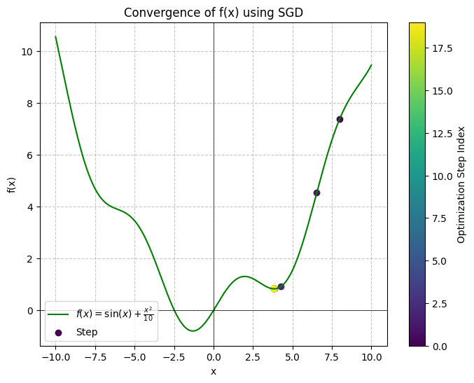
Cell output:

x: 8.0000, y: 7.3894, dy/dx: 1.4545, manual dy/dx: 1.4545
x: 6.5455, y: 4.5437, dy/dx: 2.2749, manual dy/dx: 2.2749
...
x: 3.8375, y: 0.8316, dy/dx: 0.0000, manual dy/dx: 0.0000
Diff: 5.14391, x: 3.83747, f(x): 0.83156, optimum: -1.30644, f(optimum): -0.79458
We failed to converge after 20 steps!

As we can see, we end up converging in the local minimum at $x = 3.83747$ instead of the true global minimum at $- 1.30644$ . So how can we resolve this? Let’s look at the next optimizer.

SGD With Momentum

In naive SGD, each update step happens discretely by simply looking at which way the curve is changing at that point in time and moving in the direction best suited for our optimization (in the $+$ direction for a maximization, and $-$ for a minimization). But we actually have a lot of data built up from our previous steps which we don’t end up making use of.

Physics Refresher

Recall that in physics, we had the following equations to describe the change in the position of an object:

Position:

x_{f} Δ x = x_{0} + Δ x = x_{f} - x_{0} new position as a result of positional difference change in position

Where:

$x_{0}$ is the initial position
$x_{f}$ is the final position
$Δ x$ is the change in position

And we found that if we considered the time associated with the positional change, we were able to calculate the rate of change of the position with respect to time $t$ :

Δ t = t_{f} - t_{i} \frac{Δ x}{Δ t}

Where:

$t_{0}$ is the initial time
$t_{f}$ is the final time
$Δ t$ is the change in time

We could then calculate the velocity as a function of the change in position over time:

Velocity:

v ∴ v = \frac{x _{f} - x _{0}}{t _{f} - t _{0}} = \frac{Δ x}{Δ t}

Where:

$v$ is the particle’s velocity

And using this information, this gave us information about the particle’s rate of change over time.

We were then able to express the position of the particle as a function of time $x (t)$ by the following equation:

x (t) = x_{0} + v t

Acceleration:

Since velocity changes over time, we represent and quantify this value $a$ as acceleration and describe it as follows:

Δ v a = v_{f} - v_{0} = \frac{Δ v}{Δ t} acceleration change in velocity

Where:

$v_{0}$ is the particle’s initial velocity
$v_{f}$ is the particle’s final velocity
$Δ v$ is the average change in velocity
$a$ is the particle’s acceleration

We can then therefore express the velocity also as a function of time $t$ :

v (t) = v_{0} + a t

Bringing Physics into Optimization

If we go back to the previous example, we can see that at each step we actually have some information about where we are headed pertinent to the landscape. Here are the first few update steps when we begin optimizing:

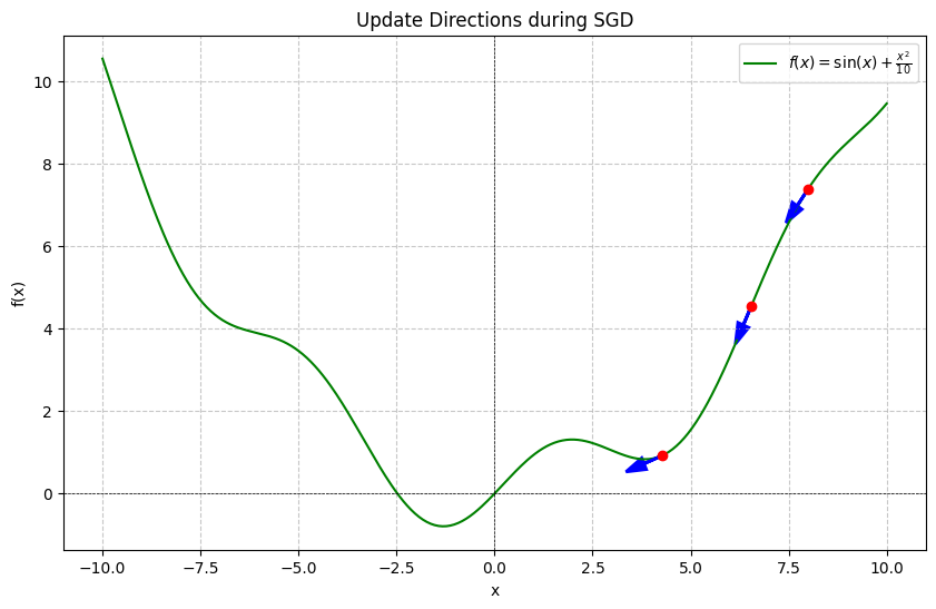
In some sense, we are going downhill and therefore can probably serve to store our history in order to build up momentum during our optimization. We can do that by making the following adjustments:

Introduce Velocity:

First, let’s introduce a velocity term $v_{t}$ at each step which will track our overall movement. Since at the start of our optimization we essentially are beginning from rest, it follows that the initial velocity can be set to zero:

v_{0} = 0

And as we’ve defined previously by the change in velocity formula, where $v (t) = v_{0} + a t$ , we can adjust this definition if we assign $a$ to be our gradient $g (θ_{t})$ and $t$ to be our learning rate $η$ .

Then, we can define the velocity update for a time $t$ using the information from the current step using the given formula:

v_{t + 1} \leftarrow μ v_{t} + (- g (θ_{t})) η

And therefore can be written as:

v_{t + 1} \leftarrow μ v_{t} - η g (θ_{t})

Since we are minimizing the gradient, we substitute the acceleration term with the negative gradient: $- g (θ_{t})$ .

We also introduce a momentum term $μ$ which controls how much the past velocity affects the present update. $μ$ is a hyperparameter which is usually set to $0.9$ or $0.99$ .

Update Rule

We define the update rule for SGD with Momentum as:

v_{0} v_{t + 1} θ_{t + 1} \leftarrow 0 \leftarrow μ v_{t} - η g (θ_{t}) \leftarrow θ_{t} + v_{t + 1} initialize velocity velocity update parameter update rule

Where:

$v_{0}$ is the initial velocity, typically initialized to 0
$v_{t}, v_{t + 1}$ is the velocity at step $t$ and $t + 1$ respectively
$μ$ is the momentum term, typically set to $0.9$
$η$ is our learning rate
$g (θ_{t})$ is the gradient at step $t$

Implementation

Here’s what the implementation of SGD with momentum looks like in the context of PyTorch:

import torch
from torch.nn import Parameter
from typing import Iterable

class SGDWithMomentum:
  def __init__(self, params: Iterable[Parameter], lr = 1e-1, momentum = 0.9):
    self.params = [p for p in params]
    self.velocity = [torch.zeros_like(p) for p in self.params]
    self.lr = lr
    self.momentum = momentum

  @torch.no_grad()
  def step(self):
    for i, p in enumerate(self.params):
      self.velocity[i] = self.momentum * self.velocity[i] - self.lr * p.grad.data
      p.data = p.data + self.velocity[i]

  def zero_grad(self, set_to_none = True):
    for p in self.params:
      p.grad = None

Memory & Compute Analysis

SGD + Momentum serves as the first optimizer where our resource requirements increase from plain SGD. Our compute requirement is still $O (N)$ since all of our computations are element-wise, and we don’t do any other nesting.

But our memory increases to $O (N)$ compared to $O (1)$ of vanilla SGD, since we are now having to store a momentum variable for each parameter the model has.

The implications are now that if you have a model with 1,000 parameters in FP16 (2 bytes / parameters), you would need enough memory for the following:

Model Parameters: $1, 000 \times 2 B = 2 kB$
Model Gradients: $1, 000 \times 2 B = 2 kB$
Momentum: $1, 000 \times 2 B = 2 kB$
Total: $6 kB$

Similarly, for a model 1 billion parameter model, this requirement would become:

Model Parameters: $1, 000, 000, 000 \times 2 B = 2 GB$
Model Gradients: $1, 000, 000, 000 \times 2 B = 2 GB$
Momentum: $1, 000, 000, 000 \times 2 B = 2 GB$
Total: $6 GB$

Meaning you would need 6GB of memory just to be able to load the model memory. Typically for large models like transformers, this requirement is much higher.

Examples

Using the above implementation, let’s see what happens when we apply it to finding the global optima of $f (x) = s in (x) + x^{2} /10$ .

Using the new optimizer, our code hardly changes:

import torch

# Set manual seed for reproducibility
torch.manual_seed(42)

# Define the function to optimize
def f(x) -> torch.Tensor:
    return torch.sin(x) + (x**2) / 10

# Initialize optimization parameters
learning_rate = 0.1
momentum = 0.9
x = torch.tensor([8.0], requires_grad=True, dtype=torch.float32)  # Starting point
optimizer = SGDWithMomentum([x], lr=learning_rate, momentum=momentum)

# Define the actual answer and tolerance for convergence
actual_answer = torch.tensor([-1.30644])
tolerance = 1e-6

# Number of optimization steps
N = 1000
xs, ys = [], []
gradients = []  # To store gradients for arrow visualization
deltas = []     # To store delta_x and delta_y for arrows

for i in range(N):
    optimizer.zero_grad()    # Reset gradients
    y = f(x)                 # Compute function value
    xs.append(x.detach().item())
    ys.append(y.detach().item())
    
    y.backward()            # Backpropagate to compute gradients
    with torch.no_grad():
        dy_dx = torch.cos(x) + x / 5  # Manual gradient computation
        gradient = dy_dx.item()      # Store gradient value
        gradients.append(gradient)    # Append to gradients list
        if i % 100 == 0:
          print(f'Step {i+1}: x = {x.item():.4f}, f(x) = {y.item():.4f}, dy/dx = {x.grad.data.item():.4f}, manual dy/dx = {dy_dx.item():.4f}')
        
        # Compute delta_x and delta_y based on the optimizer's step
        delta_x = -learning_rate * gradient  # Actual parameter update (SGD step)
        # Since f(x) = sin(x) + x^2/10, the change in y can be approximated as:
        # delta_y ≈ f'(x) * delta_x = gradient * delta_x
        delta_y = gradient * delta_x
        deltas.append( (delta_x, delta_y) )
        
        # Check for convergence
        if (diff := abs(x - actual_answer)) <= tolerance:
            print(f"Converged after {i+1} steps!")
            break
    
    optimizer.step()         # Update parameters

# After optimization steps
with torch.no_grad():
    final_diff = abs(x - actual_answer).item()
    final_x = x.item()
    final_y = f(x).item()
    print(f"\nFinal Results:")
    print(f"Diff: {final_diff:.5f}, x: {final_x:.5f}, f(x): {final_y:.5f}")
    if final_diff <= tolerance:
        print(f"We've converged after {i+1} steps!")
    else:
        print(f"We did not converge after {N} steps.")

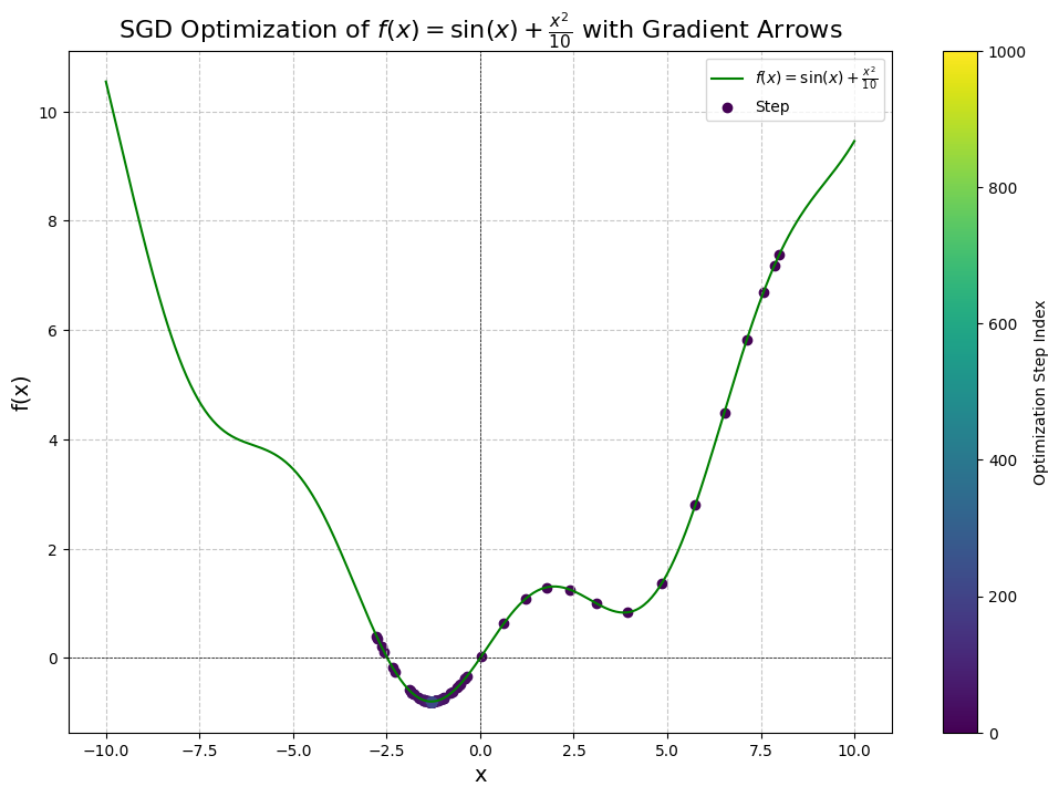
The output we get is a bit interesting, notice how many steps it has taken us:

Step 1: x = 8.0000, f(x) = 7.3894, dy/dx = 1.4545, manual dy/dx = 1.4545
Step 101: x = -1.2908, f(x) = -0.7944, dy/dx = 0.0182, manual dy/dx = 0.0182
Step 201: x = -1.3065, f(x) = -0.7946, dy/dx = -0.0001, manual dy/dx = -0.0001
Converged after 216 steps!

Final Results:
Diff: 0.00000, x: -1.30644, f(x): -0.79458
We've converged after 216 steps!

Click to view the full cell

# Function plot data
x_values = np.linspace(-10, 10, 400)
y_values = np.sin(x_values) + (x_values ** 2) / 10

# Set up the plot
fig, ax = plt.subplots(figsize=(12, 8))

# Plot the function f(x)
ax.plot(x_values, y_values, label=r'$f(x) = \sin(x) + \frac{x^2}{10}$', color='green')

# Use a colormap for the optimization steps
norm = plt.Normalize(0, N)
cmap = plt.cm.viridis
colors = cmap(norm(range(len(xs))))

# Scatter points with gradient colors
for i in range(len(xs)):
    ax.scatter(xs[i], ys[i], color=colors[i], label='Step' if i == 0 else "")

# Add colorbar to represent step index
sm = ScalarMappable(cmap=cmap, norm=norm)
sm.set_array([])
cbar = fig.colorbar(sm, ax=ax)
cbar.set_label('Optimization Step Index')


# Enhance plot aesthetics
ax.set_xlabel('x', fontsize=14)
ax.set_ylabel('f(x)', fontsize=14)
ax.set_title('SGD Optimization of $f(x) = \sin(x) + \\frac{{x^2}}{10}$ with Gradient Arrows', fontsize=16)
ax.axhline(0, color='black', linewidth=0.5, linestyle='--')
ax.axvline(0, color='black', linewidth=0.5, linestyle='--')
ax.grid(True, linestyle='--', alpha=0.7)
ax.legend()
plt.show()

So we were able to solve the problem of getting stuck in a local minima, although it took us 216 steps* to reach the global minimum of this function from the right side. While it seems like a lot, this is actually a very good result considering we are initializing poorly.

Let me illustrate a few more examples.

$sin (x) + x^{2} /10$ from the left side

Revisiting our previous example, let’s see what happens when we use our new method on the convergence from the left side:

Step 1: x = -8.0000, f(x) = 5.4106, dy/dx = -1.7455, manual dy/dx = -1.7455
Step 101: x = -1.2936, f(x) = -0.7945, dy/dx = 0.0150, manual dy/dx = 0.0150
Step 201: x = -1.3064, f(x) = -0.7946, dy/dx = 0.0001, manual dy/dx = 0.0001
Converged after 222 steps!

Final Results:
Diff: 0.00000, x: -1.30644, f(x): -0.79458
We've converged after 222 steps!

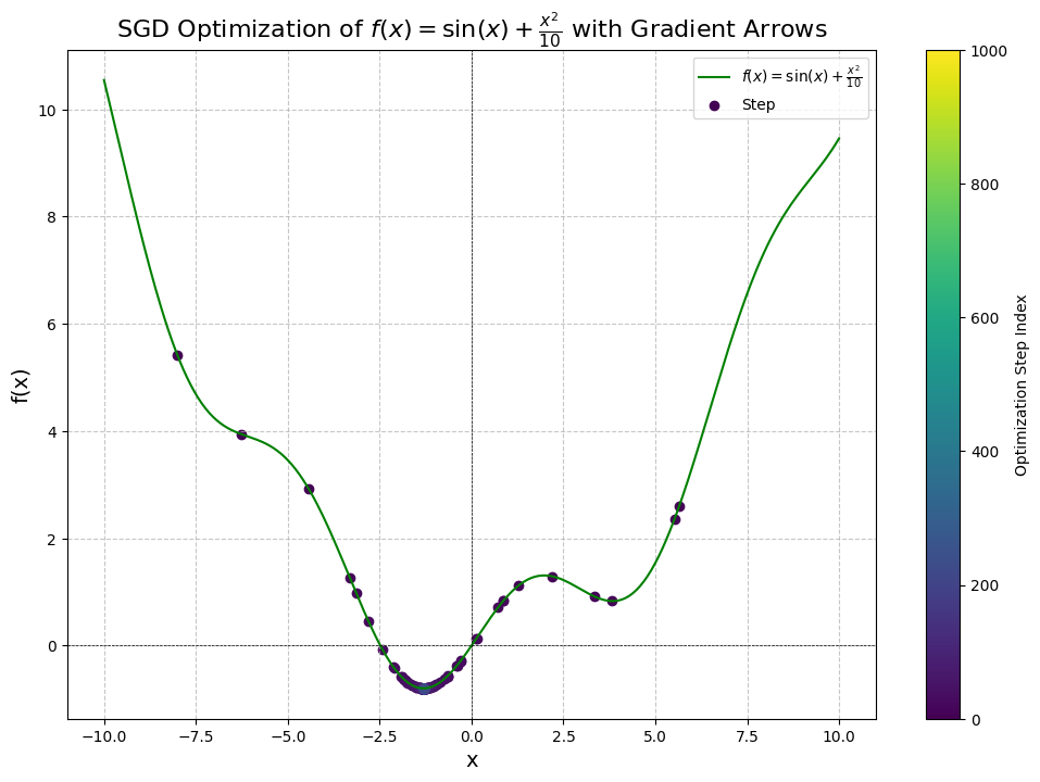
As we can see from this curve, it now took us 222 steps using the same hyper-parameters $η = 1.0$ as last time, with $μ = 0.9$ as the new hyper-parameter. To understand why, let’s inspect the curve a little more.

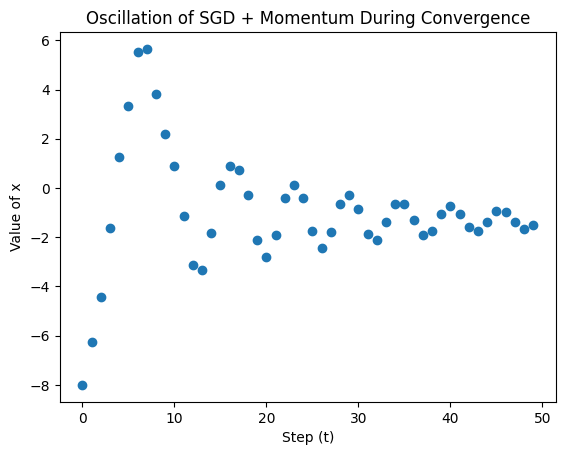
Although we started on the left side, we see that there are actually a few dots on the right-hand side of the minimum, near the local minima. The momentum from our gradients actually ended up overshooting the global minimum and caused us to keep moving back up the hill and towards the other local minima before descending back down.

The problem we are facing is called oscillation and is defined as follows:

Definition: Oscillation

The phenomenon where the parameters being optimized fluctuate back and forth without settling into a stable optimization.

To illustrate this point, let’s plot out the first 50 steps during optimization:

Click to view the full cell

import numpy as np
window = 50
t = list(range(len(xs[:window])))
t
plt.title("Oscillation of SGD + Momentum During Convergence")
plt.xlabel('Step (t)')
plt.ylabel('Value of x')
plt.scatter(t, xs[:window])

The reason is that by adding a velocity term, we start following newton’s first law of motion:

Newton’s Law of Inertia: An object in motion remains in motion unless acted upon.

This means that our convergence will be dependent on proper initialization and careful selection of our hyperparameters.

To solve this issue, let’s take a look at the next optimizer.

Nesterov’s Accelerated Gradient

In our previous example, we were updating the gradient in such a way that we were adding the velocity $μ v_{t}$ at time in addition to the gradient $- η g (θ_{t})$ .

As described in a paper by Ilya Sutskever Et. Al, On the importance of initialization and momentum in deep learning, the effect that this has geometrically is the resulting parameters $θ_{t + 1}$ may end up in a position where the resulting gradient $g (θ_{t + 1})$ was overshot and is therefore moving back into the opposite direction from the previous update.

To understand this, consider the following graphic:

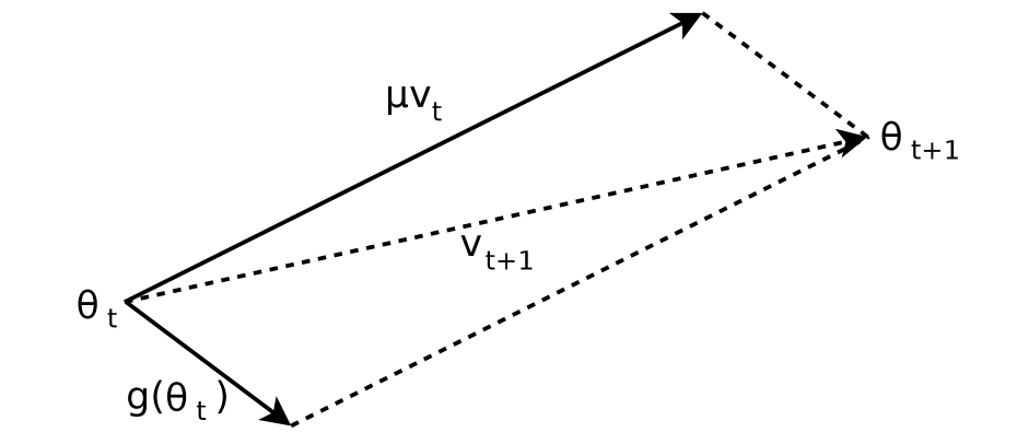
We see here that at $θ_{t}$ the $\overset{y}{^}$ component of $g (θ_{t})$ is of the opposite sign to the moment $μ \overset{v_{t}}{^}$ , i.e: $g (θ_{t})_{y} < 0 < \overset{v}{^}_{t y}$ . This results in a suboptimal gradient update in which the momentum overpowers the gradient and pushes us into the suboptimal direction for $\overset{y}{^}$ .

What Nesterov’s Accelerated Gradient (NAG) proposes is the following: rather than adding the momentum after the gradient computation at $t$ , what if we instead added the momentum before the gradient computation? That is — rather than fighting with the momentum, we instead look to where the momentum would move the parameter, and then compute the gradient at that point before applying the update rule.

In other words, the update rule for $v_{t}$ becomes:

v_{t + 1} \leftarrow μ v_{t} - η g (θ_{t} + μ v_{t})

Graphically, this has the following effect:

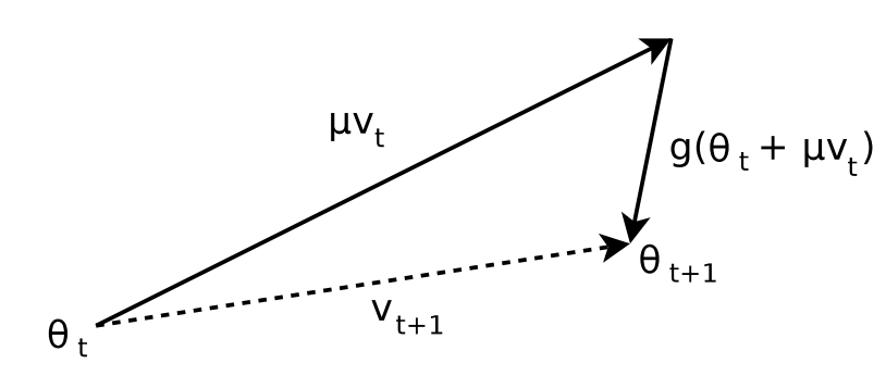
In other words, we replace the input to the gradient calculation from $θ_{t}$ to $θ_{t}^{*}$ such that:

θ_{t}^{*} \leftarrow μ v_{t} + θ_{t}

We then refer to this as the lookahead value for the gradient computation.

And the momentum update can instead be thought of as:

v_{t + 1} \leftarrow μ v_{t} - η g (θ_{t}^{*})

Explanation:

Since the momentum will move us to certain point regardless of what the gradient is, it’s possible that at time $t$ , the gradient may be drowned out by the momentum and therefore the parameter will be moved into a direction that we don’t like. To counteract this, we simply adjust the where the gradient is calculated in order to treat the update step as a logical sequence as if a path was being traversed intelligently.

Update rule:

Here’s the full update rule for NAG is shown below:

θ_{t}^{*} v_{t + 1} θ_{t + 1} \leftarrow μ v_{t} + θ_{t} \leftarrow μ v_{t} - η g (θ_{t}^{*}) \leftarrow θ_{t} + v_{t + 1}

Where:

$θ_{t}$ is the set of parameters at time $t$
$θ_{t}^{*}$ is the updated lookahead parameter on which the gradient will be calculated
$v_{t}, v_{t + 1}$ is the velocity at time $t$ and $t + 1$ respectively
$μ$ is the momentum factor, typically set to $0.9$
$g (θ_{t}^{*})$ is the gradient computed at the lookahead step

Implementation Details:

Due to how the gradient is computed with this optimizer compared to others, there are many different implementations of NAG. There’s a great website created by James Melville which provides an in-depth look at various implementations of NAG. In his summary after analyszing all of the various optimizers he states:

In terms of implementation, I pity anyone tasked with implementing Nesterov momentum and demonstrating that they actually got it right.

In this article I will show just two implementations. The one based on the above formulation, and the one used by PyTorch. This optimizer in particular is the only one in this article we’ll cover which suffers from this problem.

To solve $sin (x) + x^{2} /10$ :

We can implement the NAG update rule as follows:

import torch

def f(x) -> torch.Tensor:
  return torch.sin(x) + x**2 / 10

learning_rate = 1.0
N = 1000
learning_rate = 1.0
momentum = 0.9
velocity = 0
initial_point = -8.0
x = torch.tensor([initial_point], requires_grad=True, dtype=torch.float32)  # Starting point

# Define the actual answer and tolerance for convergence
actual_answer = torch.tensor([-1.30644])
tolerance = 1e-6

# Number of optimization steps
N = 1000
xs, ys = [], []
gradients = []  # To store gradients for arrow visualization
deltas = []     # To store delta_x and delta_y for arrows

for i in range(N):
    # zero gradients
    x.grad = None

    # nesterov gradient calculation
    x_old = x.detach().clone()
    x.data = x.data + momentum * velocity

    # computes df/d(theta + mu * v)
    y = f(x)                 
    xs.append(x.detach().item())
    ys.append(y.detach().item())

    # Backpropagate to compute gradients
    y.backward()            
    with torch.no_grad():
        dy_dx = torch.cos(x_old + momentum * velocity) + (x_old + momentum * velocity) / 5
        gradient = dy_dx.item()      # Store gradient value
        gradients.append(y.data.detach())    # Append to gradients list
        if i % 100 == 0:
          print(f'Step {i+1}: x = {x.item():.4f}, f(x) = {y.item():.4f}, dy/dx = {x.grad.data.item():.4f}, manual dy/dx = {dy_dx.item():.4f}')
        
        # Check for convergence
        if (diff := abs(x - actual_answer)) <= tolerance:
            print(f"Converged after {i+1} steps!")
            break

    # update rule
    with torch.no_grad():
        velocity = momentum * velocity - learning_rate * x.grad.data
        x.data = x_old + velocity



# After optimization steps
with torch.no_grad():
    final_diff = abs(x - actual_answer).item()
    final_x = x.item()
    final_y = f(x).item()
    print(f"\nFinal Results:")
    print(f"Diff: {final_diff:.5f}, x: {final_x:.5f}, f(x): {final_y:.5f}")
    if final_diff <= tolerance:
        print(f"We've converged after {i+1} steps!")
    else:
        print(f"We did not converge after {N} steps.")

And here are the results we get:

Step 1: x = -8.0000, f(x) = 5.4106, dy/dx = -1.7455, manual dy/dx = -1.7455
Converged after 34 steps!

Final Results:
Diff: 0.00000, x: -1.30644, f(x): -0.79458
We've converged after 34 steps!

As we can see, the convergence only takes 34 steps compared to the previous results of naive SGD + momentum of 222 steps using the same hyper-parameters.

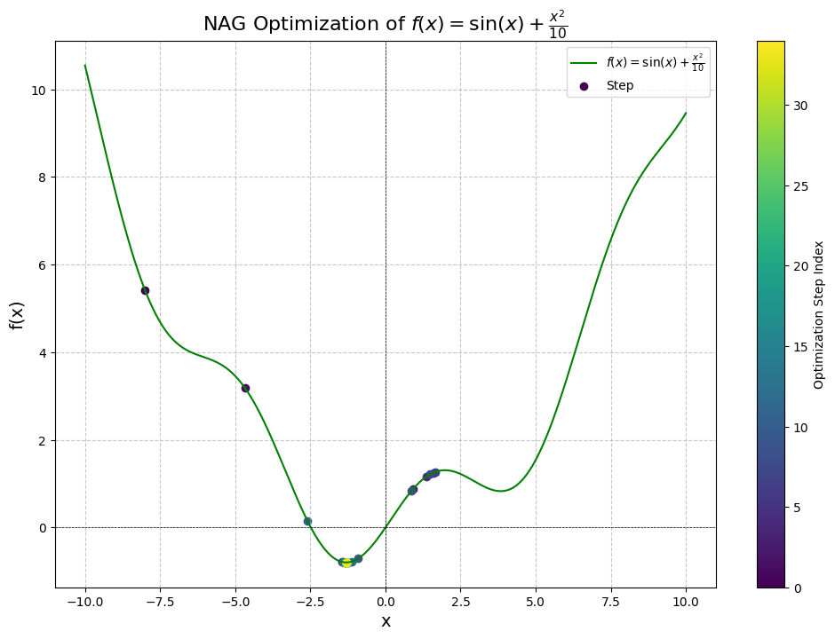
Let’s also see what happens when we approach from the right, with initial point at $x = 8$ :

Step 1: x = 8.0000, f(x) = 7.3894, dy/dx = 1.4545, manual dy/dx = 1.4545
Converged after 27 steps!

Final Results:
Diff: 0.00000, x: -1.30644, f(x): -0.79458
We've converged after 27 steps!

Here we get even better results: convergence in just 27 steps. In terms of improvement, this improved our convergance by an order of magnitude! Now we can have momentum to avoid local minima and have fast convergence for this particular problem.

In general, the best choice of optimizer will depend on the particular problem at hand, so it’s always worth experimenting and seeing what works.

PyTorch Implementation of NAG

Since NAG relies on computing the gradient with a modified set of parameters, this often doesn’t play nice with how frameworks like to separate the gradient computation from the optimizer step. As a result, popular frameworks such as PyTorch like to approximate the calculation.

In particular, the PyTorch implementation approximates the computation by doing the following update rule:

v_{0} v_{t + 1} θ_{t + 1} \leftarrow g (θ_{0}) \leftarrow μ v_{t} + g (θ_{t}) \leftarrow θ_{t} - η (g (θ_{t}) + μ v_{t + 1})

Where:

$v_{0}$ is the initial velocity, set to the first gradient
$v_{t}, v_{t + 1}$ is the velocity at time $t$ and $t + 1$
$μ$ is the momentum, often set to $0.9$
$η$ is the learning rate
$g (θ_{t})$ is the gradient at time $t$

Here’s how we would implement this version:

import torch
from torch.nn import Parameter
from typing import Iterable

class NAG:
  def __init__(self, params: Iterable[Parameter], learning_rate = 0.001, momentum = 0.9):
    self.params = [p for p in params]
    self.velocity = [None for _ in params]
    self.lr = learning_rate
    self.momentum = momentum

  @torch.no_grad()
  def step(self):
    for i, p in enumerate(self.params):
      if self.velocity[i] is None:
        self.velocity[i] = p.grad.data.clone().detach()
      else:
        self.velocity[i] = self.velocity[i] * self.momentum + p.grad.data
      p.data = p.data - self.lr * (p.grad.data + self.velocity[i] * self.momentum)

  def zero_grad(self, set_to_none=True):
    for p in self.params:
      p.grad = None

Now let’s test this one out:

Click to view implementation

import torch

def f(x) -> torch.Tensor:
  return torch.sin(x) + x**2 / 10

learning_rate = 1.0
N = 1000
learning_rate = 1.0
momentum = 0.9
velocity = 0
initial_point = 8.0
x = torch.tensor([initial_point], requires_grad=True, dtype=torch.float32)  # Starting point
optimizer = NAG([x], learning_rate, momentum)

# Define the actual answer and tolerance for convergence
actual_answer = torch.tensor([-1.30644])
tolerance = 1e-6

# Number of optimization steps
N = 1000
xs, ys = [], []

for i in range(N):
    optimizer.zero_grad()
    # computes df/d(theta + mu * v)
    y = f(x)                 
    xs.append(x.detach().item())
    ys.append(y.detach().item())
    y.backward()            # Backpropagate to compute gradients
    with torch.no_grad():
        if i % 100 == 0:
          print(f'Step {i+1}: x = {x.item():.4f}, f(x) = {y.item():.4f}, dy/dx = {x.grad.data.item():.4f}')
        
        # Check for convergence
        if (diff := abs(x - actual_answer)) <= tolerance:
            print(f"Converged after {i+1} steps!")
            break

    # update step
    optimizer.step()

# After optimization steps
with torch.no_grad():
    final_diff = abs(x - actual_answer).item()
    final_x = x.item()
    final_y = f(x).item()
    print(f"\nFinal Results:")
    print(f"Diff: {final_diff:.5f}, x: {final_x:.5f}, f(x): {final_y:.5f}")
    if final_diff <= tolerance:
        print(f"We've converged after {i+1} steps!")
    else:
        print(f"We did not converge after {N} steps.")

Results:

Step 1: x = 8.0000, f(x) = 7.3894, dy/dx = 1.4545
Converged after 27 steps!

Final Results:
Diff: 0.00000, x: -1.30644, f(x): -0.79458
We've converged after 27 steps!

Graph:

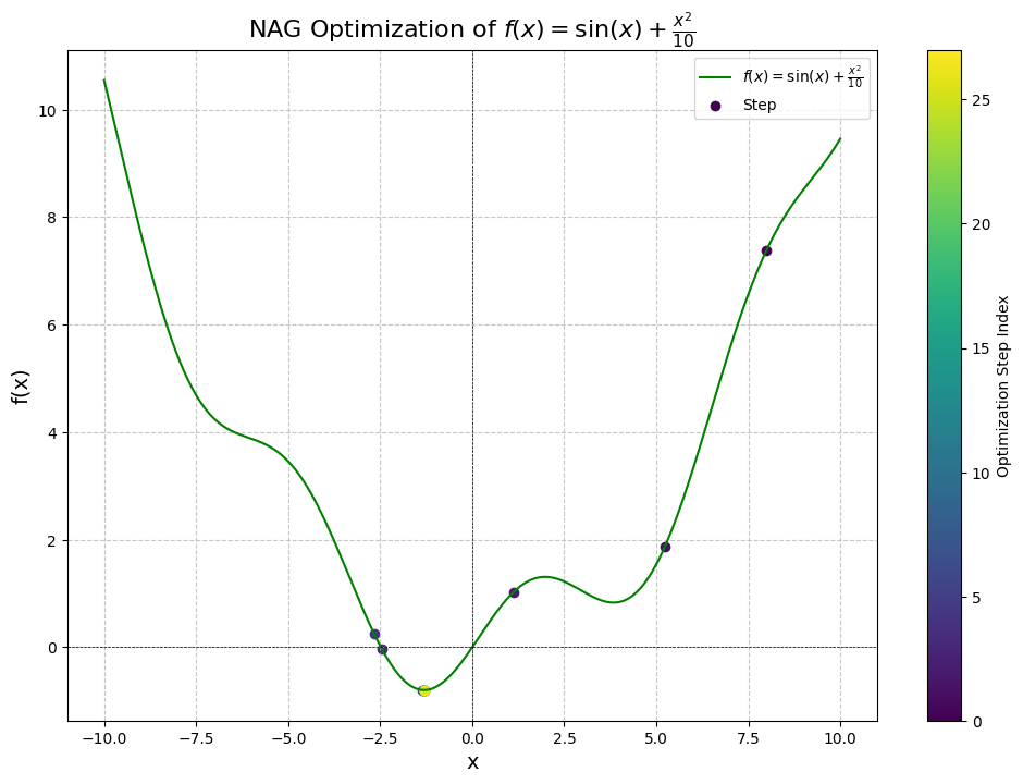
Comparing this against the built-in PyTorch implementation, we get identical results:

+ from torch.optim import SGD
...
learning_rate = 1.0
momentum = 0.9
velocity = 0
initial_point = 8.0
x = torch.tensor([initial_point], requires_grad=True, dtype=torch.float32)  # Starting point
- optimizer = NAG([x], learning_rate=learning_rate, momentum=momentum)
+ optimizer = SGD([x], lr=learning_rate, momentum=momentum, nesterov=True)
...
for i in range(N):
    optimizer.zero_grad()
    y = f(x)                 
    y.backward()            
    optimizer.step()
...

Results:

Step 1: x = 8.0000, f(x) = 7.3894, dy/dx = 1.4545
Converged after 27 steps!

Final Results:
Diff: 0.00000, x: -1.30644, f(x): -0.79458
We've converged after 27 steps!

From the few above experiments, we observe that NAG yields far superior results compared to SGD and vanilla SGD + Momentum.

The reason that NAG is so much more effective is due to its incorporation of the lookahead term which allows the optimization to be much more adaptive to the curvature of the loss landscape.

Memory & Compute Analysis

NAG requires $O (N)$ memory since we must also store the momentum for each parameter. It also only requires $O (N)$ compute since we only compute element-wise calculations in order to obtain the momentum and perform the update.

So all of the requirements we’ve established for SGD + momentum in terms of compute and memory still hold with NAG.

Conclusion

In this article, we have gone over the basics of optimization, looked at a few different loss functions & optimization problems, and developed our intuition for what optimization algorithms are accomplishing. We have also looked at a few variants of the Stochastic Gradient Descent algorithm and implemented them to solve a few problems: finding the global minimum of $f (x) = sin (x) + x^{2} /10$ , and minimizing the error of a linear regression.

We saw that SGD allows us to descend down the loss landscape in discrete steps, but suffers the problem of getting caught in local minima. We then improved upon this by accumulating gradients from our past updates and incorporating them in the update step as momentum. We also observed how doing this naively led to a high amount of oscillation which resulted in us taking much longer to converge at the global minimum. We then saw that this could be resolved by incorporating a lookahead step which evaluates the gradient at the point the parameters will be once moved by the momentum and using that instead of the gradient prior to the momentum’s movement.

So far, the optimizers we’ve looked at have only improved upon SGD by solving the issue of getting stuck in a local minimum, and particularly by adding a momentum term to the update rule. But this approach has its limitations, in particular it treats the step size for each parameter identical. In the next section, we’ll see how to address this challenge. In particular, we will build out the adaptable learning-rate optimizers, and see how all of the optimizers in the blogs perform on deep learning tasks.

References

Ilya Sutskever Et. Al - On the importance of initialization and momentum in deep learning
Andrej Karpathy - Neural Networks: Zero to Hero
Andrej Karpathy - Yes you should understand backprop
James Melville - Implementations of Nesterov’s Accelerated Gradient
Yuri Nesterov - A method of solving a convex programming problem with convergence rate $O (\frac{1}{k ^{2}})$

From ZeRO to Hero: Rebuilding FSDP From Scratch

Introduction

Optimizers From Scratch

Introduction

Why optimize?

Optimization in Machine Learning

Loss Functions: How do they work?

Example: Linear Regression

Analyzing Convergence

Gradient Descent

Stochastic Gradient Descent

Memory & Compute Analysis

Drawbacks of SGD

SGD With Momentum

Physics Refresher

Bringing Physics into Optimization

Update Rule

Implementation

Memory & Compute Analysis

Examples

sin(x)+x2/10 from the left side

Nesterov’s Accelerated Gradient

PyTorch Implementation of NAG

Memory & Compute Analysis

Conclusion

References

$sin (x) + x^{2} /10$ from the left side