asdfa

From ZeRO to Hero: Rebuilding FSDP From Scratch

Introduction

By the end of this series you will have seen how to implement your own version of FSDP that can perform distributed training. But to do this effectively, we will need to break up the series in order to understand the following foundational concepts:

Foundations of Optimization
Memory Management Techniques in Optimization
Distributed Data Parallelism
Memory Optimization in Distributed Training
Model Parallelism
ZeRO principles
FSDP

In this blog we will cover the foundations of optimization in Deep Learning. By the end of this blog, you will learn about the following optimizers, the intuition behind them, and how to rebuild them from scratch:

Stochastic Gradient Descent (SGD)
SGD with Momentum
Nesterov’s Accelerated Gradient
Adagrad
RMSProp
Adam
AdamW

Note: This series is inspired by Andrej Karpathy’s Neural Networks: Zero to Hero series. It’s recommended but not required to go through that first as it builds intuition for neural networks in the first place.

Recommended pre-requisites for this series:

To get the most value out of this series, I highly advise the following pre-requisites:

Some Calculus understanding, specifically about derivatives
Python background
Some understanding of neural networks

Optimizers From Scratch

In the world of machine learning and deep learning, we have a variety of different model architectures which all warrant their own techniques for how they actually learn. However; the training loop is the one thing which is largely universal:

""" high-level psuedocode """

model = Model()
optimizer = Optimizer(model.parameters())

for data in dataset:
  optimizer.zero_grad()
  
  # forward-pass
  loss = model(data)
  
  # backward pass
  loss.backward()

  # optimization step
  optimizer.step()

Although some models like Generative Adversarial Networks (GANs) and Reinforcement Learning (RL) models have slight alterations, we ultimately still use some form of the above training loop.

In many modern applications of deep learning, we typically instantiate some optimizer such as AdamW and simply call loss.backward() and optimizer.step(), then sit back and watch the loss curve decrease over time. However; as Andrej Karpathy pointed out in his blog Yes you should understand backprop:

it is easy to fall into the trap of abstracting away the learning process — believing that you can simply stack arbitrary layers together and backprop will “magically make them work” on your data.

While his focus was on the actual backpropagation steps, I’d argue the same is true for optimizers since each comes with its own upsides & drawbacks, so understanding why we’d want to use one over the other will make us into better engineers.

Why optimize?

The following section dives into the fundamentals of neural networks and optimization. You may skip this section if you’re just interested in the code.

Before we can build our own optimizers, we must understand what problem they’re solving and why they are so important in training deep neural networks.

If you remember back in Calculus, we were often given a function $f(x) = x^2$ and asked to evaluate its minimum. Algebraically this was simple to do, all you’d do is compute its derivative and solve for 0:

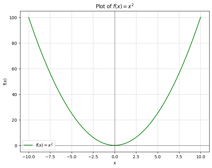
\begin{align*} f(x) &= x^2 \\ f'(x) &= 2x &\text{ power rule}\\ f'(x) &= 0 &\text{now we have to solve for }f'(x) = 0 \\ 2x &= 0 &\text{} \\ x &= 0 &\therefore f \text{ has a minimum at 0 } \\ \end{align*}

And we were often satisfied by this, since it made sense geometrically:

Here we can just look and see that the function is strictly increasing and therefore has a global minimum at $x=0$ .

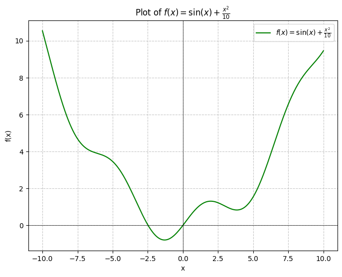
But now what if we wanted to find the global minimum of the function $f(x) = \sin(x) + \frac{x^2}{10}$ ?:

Geometrically we can see that there is clearly a global minimum (in the context of our graph) somewhere around -1, but this isn’t a satisfying enough answer. And what if a slight error here resulted in a rocket landing properly versus crashing into the ocean? We ought to have a better method of finding the answer. Let’s try to do so analytically:

\begin{align*} f(x) &= \sin(x) + \frac{x^2}{10} \\ \frac{df(x)}{dx} &= \frac{d}{dx}\left[\sin(x) + \frac{x^2}{10}\right] \\ \frac{df(x)}{dx} &= cos(x) + \frac{x}{5} \\ \end{align*}

And then solving for $f'(x) = 0$ :

\begin{align*} \frac{df(x)}{dx} &= 0 \\ cos(x) + \frac{x}{5} &= 0 \\ cos(x) &= -\frac{x}{5} \\ x &= \cos^{-1}(-\frac{x}{5}) \\ \end{align*}

Well… that’s awkward. We can’t simply find the exact global minimum of this function by solving for $f'(x) = 0$ .

At this point is where we start developing numerical methods which can allow us to find the minimum of the function. One particular method of accomplishing this is Newton’s method.

Newton’s method is a technique which allows us to approximate he roots of a real-valued function by iteratively approaching them using the following formula:

Definition: Newton’s Method

For a differentiable, real-valued function, we can iteratively approximate the roots by computing:
$x_{n+1} = x_{n} - \frac{f(x_n)}{f'(x_n)}$

So how can we use this to find the global minimum of our function? We can reframe the problem of solving $f'(x) = 0$ as finding the real-valued roots. Therefore, we can approximate the value for $x$ by getting the second derivative of $f(x)$ and plugging them into the equation. In particular, the second derivative is simply: $f''(x) = -\sin(x) + 1/5$ . So all we need to do then is compute:

x_{n+1} = x_n - \frac{f'(x_n)}{f''(x_n)}

Here’s an implementation of this in Python:

import numpy as np

def fprime2(x):
  # second derivative
  return -np.sin(x) + 0.2

def fprime(x): 
  return np.cos(x) + x / 5

def f(x):
  return np.sin(x) + (x**2) / 10

def newtons(xi, n):
  x = xi
  for i in range(n):
    fx = f(x)
    fxprime = fprime(x)
    fxprime2 = fprime2(x)
    x = x - (fxprime / fxprime2)
    print(f'[{i}/{n}] x = {x:.8}, f(x) = {fx:.5}, f\'(x) = {fxprime:.5}, f\'\'(x) = {fxprime2:.5}')

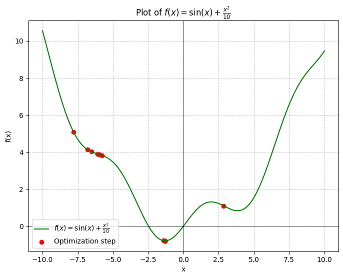
newtons(-5, 12)

>>> [0/12] x = -5.9438858, f(x) = 3.4589, f'(x) = -0.71634, f''(x) = -0.75892
>>> [1/12] x = -7.7943361, f(x) = 3.8658, f'(x) = -0.24579, f''(x) = -0.13283
>>> [2/12] x = -6.543101, f(x) = 5.0769, f'(x) = -1.4993, f''(x) = 1.1982
>>> [3/12] x = -5.7942843, f(x) = 4.0242, f'(x) = -0.34221, f''(x) = 0.457
>>> [4/12] x = -6.8178381, f(x) = 3.827, f'(x) = -0.27601, f''(x) = -0.26966
>>> [5/12] x = -6.1087584, f(x) = 4.1387, f'(x) = -0.50312, f''(x) = 0.70954
>>> [6/12] x = 2.8466056, f(x) = 3.9052, f'(x) = -0.23693, f''(x) = 0.026456
>>> [7/12] x = -1.4242582, f(x) = 1.101, f'(x) = -0.38748, f''(x) = -0.090727
>>> [8/12] x = -1.3075177, f(x) = -0.78643, f'(x) = -0.13884, f''(x) = 1.1893
>>> [9/12] x = -1.3064401, f(x) = -0.79458, f'(x) = -0.001256, f''(x) = 1.1655
>>> [10/12] x = -1.30644, f(x) = -0.79458, f'(x) = -1.513e-07, f''(x) = 1.1653
>>> [11/12] x = -1.30644, f(x) = -0.79458, f'(x) = -2.276e-15, f''(x) = 1.1653

And after 12 iterations, we find that the global minimum of $f(x) = \sin(x) + \frac{x^2}{10}$ happens to be around $x \approx -1.30644$ , which is the same as what WolframAlpha tells us.

And just like that, we have built our first-ever optimizer from scratch 😃.

Optimization in Machine Learning

Now, what does this have to do with neural networks and deep learning?

Excellent question. To understand optimizers and their relation to deep learning, we must understand what deep learning even is. Deep Learning as a subject is a subset of statistical modeling, in which we have a mathematical function $f$ which has some set of parameters $\theta$ and can predict an output $\hat{y}$ given an input $x$ . We denote this relationship as: $\hat{y} = f(x; \theta)$ .

While this may seem complex, it is really saying something simple: given an input $x$ , function $f$ will predict a value of $\hat{y}$ under the set of parameters $\theta$ .

Example: Linear regression

Let’s say we have a linear regression model: $f(x) = 2x + 5$ . The general linear regression looks like $f(x; \theta) = \theta_1 x + \theta_2$ , and so in our example we have that $\theta_1 = 2$ and $\theta_2 = 5$ .

See? This isn’t anything special, it’s just a simple $y = mx + b$ graph that we’re all used to.

If we want to make the linear regression be more accurate, we can leverage existing formulas which tell us how to get the values of $\theta_1$ and $\theta_2$ formulaically. We can use these, but we are just abstracting away the understanding of how we even optimize this function to begin with.